Usage
The package allows a quick input by the user (given in this section) and quick calculation.
Jupyter Notebooks/IPython are recommended platforms to use openpile as it provides an interactive experience.
Example 1 - Create a pile
A pile can be created in the simple following way in openpile.
>>> # import the Pile object from the construct module
>>> from openpile.construct import Pile, CircularPileSection

>>> # Create a Pile
>>> pile = Pile(name = "",
...         material='Steel',
...         sections=[
...             CircularPileSection(
...                 top=0,
...                 bottom=-10,
...                 diameter=7.5,
...                 thickness=0.07
...             ),
...             CircularPileSection(
...                 top=-10,
...                 bottom=-40,
...                 diameter=7.5,
...                 thickness=0.08
...             ),
...         ]
...     )

>>> # Print the pile data
>>> print(pile)
   Elevation [m]  Diameter [m]  Wall thickness [m]  Area [m2]     I [m4]
0            0.0           7.5                0.07   1.633942  11.276204
1          -10.0           7.5                0.07   1.633942  11.276204
2          -10.0           7.5                0.08   1.864849  12.835479
3          -40.0           7.5                0.08   1.864849  12.835479
Alternative methods can be used to create a Pile, these methods can shorten the lines of codes needed to create the pile. A pile can also be created with a custom material.
For instance, the below snippet of code with another pile made of a custom material:
>>> # create a custom material
>>> from openpile.materials import PileMaterial
>>> my_concrete = PileMaterial(
...     name="Concrete",
...     uw=24,
...     E=30e6,
...     nu=0.2,
... )

>>> # create pile
>>> p = Pile.create_tubular(
...     name="<pile name>", top_elevation=0, bottom_elevation=-40, diameter=10, wt=0.050, material=my_concrete
... )
>>> print(p)
   Elevation [m]  Diameter [m]  Wall thickness [m]  Area [m2]     I [m4]
0            0.0          10.0                0.05   1.562942  19.342388
1          -40.0          10.0                0.05   1.562942  19.342388
Once the pile (object) is created, the user can use its properties and methods to interact with it. A simple view of the pile can be extracted by printing the object as below:
The user can also extract easily the pile length, elevations and other properties.
Please see the openpile.construct.Pile
As of now, only a circular pile can be modelled in openpile, however the user can bypass the construcutor by updating the pile’s properties governing the pile’s behaviour under axial or lateral loading.
New in version 1.0.0: The user cannot anymore override the young modulus E but we can now create custom PileMaterial
via openpile.materials.PileMaterial.custom()
New in version 1.0.0: The user cannot anymore override the pile width or the second moment of area I but
we can now create a custom PileSegment object by creating a subclass of the
class openpile.materials.PileSegment.
Example 2 - Calculate and plot a p-y curve
openpile allows for quick access to soil curves. The below example shows how one can quickly calculate a soil spring at a given elevation and plot it.
The different curves available can be found in the below modules.
openpile.utils.py_curves(distributed lateral curves)openpile.utils.mt_curves(distributed rotational curves)openpile.utils.tz_curves(distributed axial curves)openpile.utils.qz_curves(base axial curves)openpile.utils.Hb_curves(base shear curves)openpile.utils.Mb_curves(base moment curves)
Here below is an example of how a static curve for the API sand model looks like. The matplotlib library can be used easily with OpenPile.
# import p-y curve for api_sand from openpile.utils
from openpile.utils.py_curves import api_sand

y, p = api_sand(sig=50, # vertical stress in kPa
                X = 5, # depth in meter
                phi = 35, # internal angle of friction
                D = 5, # the pile diameter
                below_water_table=True, # use initial subgrade modulus under water
                kind="static", # static curve
                )

# create a plot of the results with Matplotlib
import matplotlib.pyplot as plt

# use matplotlib to visual the soil curve
plt.plot(y,p)
plt.ylabel('p [kN/m]')
plt.xlabel('y [m]')

Example 3 - Create a soil profile’s layer
The creation of a layer can be done with the below lines of code. A Lateral and/or Axial soil model can be assigned to a layer.
>>> from openpile.construct import Layer
>>> from openpile.soilmodels import API_clay

>>> # Create a layer
>>> layer1 = Layer(name='Soft Clay',
...             top=0,
...             bottom=-10,
...             weight=18,
...             lateral_model=API_clay(Su=[30,35], eps50=[0.01, 0.02], kind="static"), )

>>> print(layer1)
Name: Soft Clay
Elevation: (0.0) - (-10.0) m
Weight: 18.0 kN/m3
Lateral model:   API clay
   Su = 30.0-35.0 kPa
   eps50 = 0.01-0.02
   static curves
   ext: None
Axial model: None
Example 4 - Create a soil profile
>>> from openpile.construct import SoilProfile, Layer
>>> from openpile.soilmodels import API_sand, API_clay

>>> # Create a 40m deep offshore Soil Profile with a 15m water column
>>> sp = SoilProfile(
...     name="Offshore Soil Profile",
...     top_elevation=0,
...     water_line=15,
...     layers=[
...         Layer(
...             name='medium dense sand',
...             top=0,
...             bottom=-20,
...             weight=18,
...             lateral_model= API_sand(phi=33, kind="cyclic")
...         ),
...         Layer(
...             name='firm clay',
...             top=-20,
...             bottom=-40,
...             weight=18,
...             lateral_model= API_clay(Su=[50, 70], eps50=0.015, kind="cyclic")
...         ),
...     ]
... )

>>> print(sp)
Layer 1
------------------------------
Name: medium dense sand
Elevation: (0.0) - (-20.0) m
Weight: 18.0 kN/m3
Lateral model:      API sand
    phi = 33.0°
    cyclic curves
    ext: None
Axial model: None
~~~~~~~~~~~~~~~~~~~~~~~~~~~~~~
Layer 2
------------------------------
Name: firm clay
Elevation: (-20.0) - (-40.0) m
Weight: 18.0 kN/m3
Lateral model:      API clay
    Su = 50.0-70.0 kPa
    eps50 = 0.015
    cyclic curves
    ext: None
Axial model: None
~~~~~~~~~~~~~~~~~~~~~~~~~~~~~~
Example 5 - Run a lateral pile analysis
>>> from openpile.construct import Pile, SoilProfile, Layer, Model
>>> from openpile.soilmodels import API_clay, API_sand
>>>
>>> p = Pile.create_tubular(
...     name="<pile name>", top_elevation=0, bottom_elevation=-40, diameter=7.5, wt=0.075
... )
>>>
>>> # Create a 40m deep offshore Soil Profile with a 15m water column
>>> sp = SoilProfile(
...     name="Offshore Soil Profile",
...     top_elevation=0,
...     water_line=15,
...     layers=[
...         Layer(
...             name="medium dense sand",
...             top=0,
...             bottom=-20,
...             weight=18,
...             lateral_model=API_sand(phi=33, kind="cyclic"),
...         ),
...         Layer(
...             name="firm clay",
...             top=-20,
...             bottom=-40,
...             weight=18,
...             lateral_model=API_clay(Su=[50, 70], eps50=0.015, kind="cyclic"),
...         ),
...     ],
... )
>>>
>>> # Create Model
>>> M = Model(name="<model name>", pile=p, soil=sp)
>>>
>>> # Apply bottom fixity along z-axis
>>> M.set_support(elevation=-40, Tz=True)
>>> # Apply axial and lateral loads
>>> M.set_pointload(elevation=0, Pz=-20e3, Py=5e3)
>>>
>>> # Run analysis
>>> result = M.solve()
Converged at iteration no. 2
>>>
>>> # plot the results
>>> result.plot()

Example 6 - Visualize a model
If one would like to check the input of the model, a quick visual on this
can be provided by plotting the model with the method: openpile.construct.Model.plot().
>>> # Create Model
>>> M = Model(name="<model name>", pile=p, soil=sp)
>>> # Apply bottom fixity along z-axis
>>> M.set_support(elevation=-40, Tz=True)
>>> # Apply axial and lateral loads
>>> M.set_pointload(elevation=0, Pz=-20e3, Py=5e3)
>>> # Plot the Model
>>> M.plot()

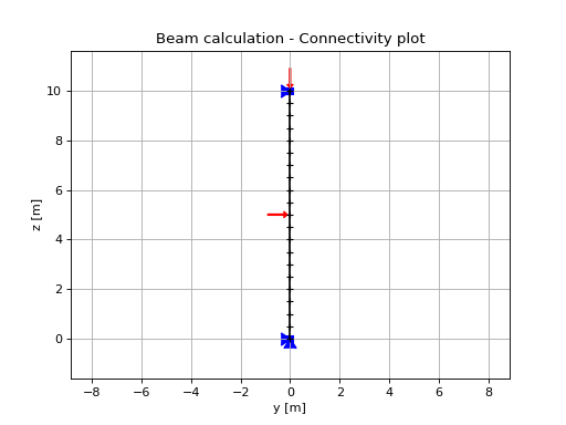
Example 7 - Run a simple beam calculation
#imports
from openpile.construct import Pile, Model
#create a tubular pile
p = Pile.create_tubular(name="Simple tubular pile", top_elevation=10, bottom_elevation=0, diameter=0.1, wt=0.01)
# create a model with this pile we just created
m = Model(name="Beam calculation", pile=p, coarseness=0.2)
# create boundary conditions
m.set_support(10, Ty=True )
m.set_support(0, Tz=True, Ty=True)
m.set_pointload(elevation=5, Py=1)
#run solver and plot result
result = m.solve()

#closed form solution is max_deflection = PL^3/(48EI)
normalized_deflection = result.deflection['Deflection [m]']*(48*p.E*p.sections[0].second_moment_of_area)/10**3
import matplotlib.pyplot as plt
_, axs = plt.subplots(nrows=1, ncols=2, figsize=(8,5))
m.plot(ax=axs[0])
axs[1].plot(normalized_deflection, result.deflection['Elevation [m]'] )
axs[1].set_xlabel("Normzalized Deflection $\delta_n=\dfrac{\delta \cdot 48 EI}{PL^3}$")
axs[1].set_ylim(axs[0].get_ylim())
axs[1].set_title('Results against\nclosed-form solution')
axs[1].grid()

Example 8 - A less simple beam calculation
#imports
from openpile.construct import Pile, Model
#create a tubular pile
p = Pile.create_tubular(name="Simple tubular pile", top_elevation=10, bottom_elevation=0, diameter=1, wt=0.1)
print(p)
# create a model with this pile we just created
m = Model(name="Beam calculation", pile=p)
# create boundary conditions with fixed rotation
m.set_support(10, Rx=True,Ty=True, )
m.set_support(0, Tz=True, Ty=True, Rx=True)
m.set_pointload(elevation=5, Py=1)
m.set_pointload(elevation=10, Pz=-1)
m.plot()
#run solver and plot result
result = m.solve()
result.plot()

Example 9 - Calculate pile settlement (axial analysis)
from openpile.construct import Pile, SoilProfile, Layer, Model
from openpile.soilmodels import API_clay_axial, API_sand_axial, API_clay, API_sand
# Create a 20m deep offshore XL pile with a 15m water column
p = Pile.create_tubular(
    name="", top_elevation=0, bottom_elevation=-20, diameter=7.5, wt=0.075
)
# Create a 20m deep offshore Soil Profile with a 15m water column
sp = SoilProfile(
    name="Offshore Soil Profile",
    top_elevation=0,
    water_line=15,
    layers=[
        Layer(
            name="medium dense sand",
            top=0,
            bottom=-20,
            weight=18,
            axial_model=API_sand_axial(delta=28),
        ),
    ],
)
# Create Model
M = Model(name="", pile=p, soil=sp)
# Apply fixity along lateral axis
M.set_support(elevation=-20, Ty=True)
M.set_support(elevation=0, Ty=True)
# Apply axial load
M.set_pointdisplacement(elevation=0, Tz=-1)
# Run analysis
result = M.solve()
result.plot_axial_results()
