API 

Construct module 

The construct module is used to construct all objects that form the inputs to calculations in openpile.

These objects include:

Pile - PileMaterial - PileSection
SoilProfile
Layer
Model

Usage

>>> from openpile.construct import Pile, SoilProfile, Layer, Model

Class openpile.construct.PileSection[source]

Bases: BaseModel, ABC

An abstract Pile Segment is a section of a pile.

abstract property top_elevation: float

abstract property bottom_elevation: float

abstract property footprint: float

abstract property length: float

abstract property area: float

abstract property entrapped_area: float

abstract property outer_perimeter: float

abstract property inner_perimeter: float

abstract get_volume(length)[source]

Return type:: float

abstract get_entrapped_volume(length)[source]

Return type:: float

abstract property width: float

abstract property second_moment_of_area: float

Class openpile.construct.CircularPileSection[source]

Bases: PileSection

A circular section of a pile.

Parameters:

top (float) – the top elevation of the circular section, in meters
bottom (float) – the bottom elevation of the circular section, in meters
diameter (float) – the diameter of the circular section, in meters
thickness (Optional[float], optional) – the wall thickness of the circular section if the section is hollow, in meters, by default None which means the section is solid.

field top: float [Required]

Validated by:

check_elevations
get_proper_thickness

field bottom: float [Required]

Validated by:

check_elevations
get_proper_thickness

field diameter: float [Required]

Validated by:

check_elevations
get_proper_thickness

field thickness: Optional[float[float]] = None

Validated by:

check_elevations
get_proper_thickness

property top_elevation: float

property bottom_elevation: float

property length: float

property area: float

property entrapped_area: float

property outer_perimeter: float

property inner_perimeter: float

property footprint: float

property width: float

property second_moment_of_area: float

get_volume(length)[source]

Return type:: float

get_entrapped_volume(length)[source]

Return type:: float

Class openpile.construct.Pile[source]

Bases: AbstractPile

field name: str [Required]

name of the pile

Validated by:

check_materials
sections_must_be_provided
sections_must_not_overlap

field sections: List[PileSection[PileSection]] [Required]

There can be as many sections as needed by the user. The length of the listsdictates the number of pile sections.

Validated by:

check_materials
sections_must_be_provided
sections_must_not_overlap

field material: Union[typing_extensions.Literal[Steel, Concrete], PileMaterial] [Required]

A class to create the pil.e.

Parameters:

name (str) – Pile/Structure’s name.
sections (List[PileSection]) – argument that stores the relevant data of each pile segment. numbering of sections is made from uppermost elevation and 0-indexed.
material (Literal["Steel",]) – material the pile is made of. by default “Steel”

Example

>>> from openpile.construct import Pile, CircularPileSection
>>> # Create a pile instance with two sections of respectively 10m and 30m length.
>>> pile = Pile(name = "",
...         material='Steel',
...         sections=[
...             CircularPileSection(
...                 top=0,
...                 bottom=-10,
...                 diameter=7.5,
...                 thickness=0.07
...             ),
...             CircularPileSection(
...                 top=-10,
...                 bottom=-40,
...                 diameter=7.5,
...                 thickness=0.08
...             ),
...         ]
...     )

One can also create a pile from other constructors such as: create_tubular(), that creates a ciruclar hollow pile of one unique section.

>>> from openpile.construct import Pile
>>> pile = Pile.create_tubular(name = "",
...         top_elevation = 0,
...         bottom_elevation = -40,
...         diameter=7.5,
...         wt=0.07,
...         )

Validated by:

check_materials
sections_must_be_provided
sections_must_not_overlap

property top_elevation: float

property data: DataFrame

property bottom_elevation: float: Bottom elevation of the pile [m VREF].

property length: float: Pile length [m].

property volume: float: Pile volume [m3].

property weight: float: Pile weight [kN].

property G: float: Shear modulus of the pile material [kPa]. Thie value does not vary across and along the pile.

property E: float: Young modulus of the pile material [kPa]. Thie value does not vary across and along the pile.

property tip_area: float: Sectional area at the bottom of the pile [m2]

property tip_footprint: float: footprint area at the bottom of the pile [m2]

property inner_volume: float: the inner volume in [m3] of the pile from the model object.

classmethod create_tubular(name, top_elevation, bottom_elevation, diameter, wt, material='Steel')[source]

A method to simplify the creation of a Pile instance. This method creates a circular and hollow pile of constant diameter and wall thickness.

Parameters:

name (str) – Pile/Structure’s name.
top_elevation (float) – top elevation of the pile [m VREF]
bottom_elevation (float) – bottom elevation of the pile [m VREF]
diameter (float) – pile diameter [m]
wt (float) – pile’s wall thickness [m]
material (Literal["Steel", "Concrete"] or an instance of openpile.materials.PileMaterial) – material the pile is made of. by default “Steel”

Returns:

a Pile instance.

Return type:

openpile.construct.Pile

property shape

Class openpile.construct.Layer[source]

Bases: AbstractLayer

A class to create a layer.

The Layer stores information on the soil parameters of the layer as well as the relevant/representative constitutive model (aka. the soil spring).

Parameters:

name (str) – Name of the layer, use for printout.
top (float) – top elevation of the layer in [m].
bottom (float) – bottom elevation of the layer in [m].
weight (float) – total unit weight in [kN/m3], cannot be lower than 10.
lateral_model (LateralModel) – Lateral soil model of the layer, by default None.
axial_model (AxialModel) – Axial soil model of the layer, by default None.
color (str) – soil layer color in HEX format (e.g. ‘#000000’), by default None. If None, the color is generated randomly.

Example

>>> from openpile.construct import Layer
>>> from openpile.soilmodels import API_clay
>>> # Create a layer with increasing values of Su and eps50
>>> layer1 = Layer(name='Soft Clay',
...            top=0,
...            bottom=-10,
...            weight=19,
...            lateral_model=API_clay(Su=[30,35], eps50=[0.01, 0.02], kind='static'),
...            )
>>> # show layer
>>> print(layer1) 
Name: Soft Clay
Elevation: (0.0) - (-10.0) m
Weight: 19.0 kN/m3
Lateral model:      API clay
    Su = 30.0-35.0 kPa
    eps50 = 0.01-0.02
    static curves
    ext: None
Axial model: None

field name: str [Required]

name of the layer, use for printout

Validated by:

check_elevations

field top: float [Required]

top elevaiton of the layer

Validated by:

check_elevations

field bottom: float [Required]

bottom elevaiton of the layer

Validated by:

check_elevations

field weight: float [Required]

unit weight in kN of the layer

Validated by:

check_elevations

field lateral_model: Optional[LateralModel] = None

Lateral constitutive model of the layer

Validated by:

check_elevations

field axial_model: Optional[AxialModel] = None

Axial constitutive model of the layer

Validated by:

check_elevations

field color: Optional[str[str]] = None

Layer’s color when plotted

Validated by:

check_elevations

model_post_init(*args, **kwargs)[source]: Override this method to perform additional initialization after __init__ and model_construct. This is useful if you want to do some validation that requires the entire model to be initialized.

Class openpile.construct.SoilProfile[source]

Bases: AbstractSoilProfile

A class to create the soil profile. A soil profile consist of a ground elevation (or top elevation) with one or more layers of soil.

Additionally, a soil profile can include discrete information at given elevation such as CPT (Cone Penetration Test) data. Not Implemented yet!

Parameters:

name (str) – Name of the soil profile, used for printout and plots.
top_elevation (float) – top elevation of the soil profile in [m VREF].
water_line (float) – elevation of the water table in [m VREF].
layers (list[Layer]) – list of layers for the soil profile.
cpt_data (np.ndarray) – cpt data table with 1st col: elevation [m], 2nd col: cone resistance [kPa], 3rd col: sleeve friction [kPa], 4th col: pore pressure u2 [kPa].

Example

>>> # import objects
>>> from openpile.construct import SoilProfile, Layer
>>> from openpile.soilmodels import API_sand, API_clay
>>> # Create a two-layer soil profile
>>> sp = SoilProfile(
...     name="BH01",
...     top_elevation=0,
...     water_line=0,
...     layers=[
...         Layer(
...             name='Layer0',
...             top=0,
...             bottom=-20,
...             weight=18,
...             lateral_model= API_sand(phi=30, kind='cyclic')
...         ),
...         Layer( name='Layer1',
...                 top=-20,
...                 bottom=-40,
...                 weight=19,
...                 lateral_model= API_clay(Su=50, eps50=0.01, kind='static'),)
...     ]
... )
>>> # Check soil profile content
>>> print(sp) 
Layer 1
------------------------------
Name: Layer0
Elevation: (0.0) - (-20.0) m
Weight: 18.0 kN/m3
Lateral model:      API sand
    phi = 30.0°
    cyclic curves
    ext: None
Axial model: None
~~~~~~~~~~~~~~~~~~~~~~~~~~~~~~
Layer 2
------------------------------
Name: Layer1
Elevation: (-20.0) - (-40.0) m
Weight: 19.0 kN/m3
Lateral model:      API clay
    Su = 50.0 kPa
    eps50 = 0.01
    static curves
    ext: None
Axial model: None
~~~~~~~~~~~~~~~~~~~~~~~~~~~~~~

field name: str [Required]

name of soil profile / borehole / location

Validated by:

check_layers_elevations
check_multipliers_in_lateral_model

field top_elevation: float [Required]

top of ground elevation with respect to the model reference elevation datum

Validated by:

check_layers_elevations
check_multipliers_in_lateral_model

field water_line: float [Required]

water elevation (this can refer to sea elevation of water table)

Validated by:

check_layers_elevations
check_multipliers_in_lateral_model

field layers: List[Layer] [Required]

soil layers to consider in the soil propfile

Validated by:

check_layers_elevations
check_multipliers_in_lateral_model

field cpt_data: Optional[ndarray] = None

Cone Penetration Test data with folloeing structure: 1st col: elevation[m], 2nd col: cone resistance[kPa], 3rd col: sleeve friction [kPa] 4th col: pore pressure u2 [kPa] (the cpt data outside the soil profile boundaries will be ignored)

Validated by:

check_layers_elevations
check_multipliers_in_lateral_model

property bottom_elevation: float: Bottom elevation of the soil profile [m VREF].

plot(ax=None)[source]

Creates a plot illustrating the stratigraphy.

Parameters:: ax (axis handle from matplotlib figure, optional) – if None, a new axis handle is created
Returns:: only return the object if assign=True
Return type:: matplotlib.pyplot.figure

Example

Class openpile.construct.BoundaryFixation[source]

Bases: BaseModel

A class to create a boundary condition where support is fixed.

Parameters:

elevation (str) – Elevation of the boundary condition [m VREF]
x (bool) – Fix the boundary condition in the x-direction
y (bool) – Fix the boundary condition in the y-direction
z (bool) – Fix the boundary condition in the z-direction

field elevation: float [Required]

field x: Optional[bool] = None

field y: Optional[bool] = None

field z: Optional[bool] = None

Class openpile.construct.BoundaryDisplacement[source]

Bases: BaseModel

A class to create a boundary condition where displacement is given.

Parameters:

elevation (str) – Elevation of the boundary condition [m VREF]
x (float) – Apply displacement in the x-direction [m]
y (float) – Apply displacement in the y-direction [m]
z (float) – Apply displacement in the z-direction [m]

field elevation: float [Required]

field x: Optional[float] = None

field y: Optional[float] = None

field z: Optional[float] = None

Class openpile.construct.BoundaryForce[source]

Bases: BaseModel

A class to create a boundary condition where force is given.

Parameters:

elevation (str) – Elevation of the boundary condition [m VREF]
x (float) – Apply force in the x-direction [kN]
y (float) – Apply force in the y-direction [kN]
z (float) – Apply force in the z-direction [kN]

field elevation: float [Required]

field x: Optional[float] = None

field y: Optional[float] = None

field z: Optional[float] = None

Class openpile.construct.Model[source]

Bases: AbstractModel

A class to create a Model.

A Model is constructed based on the pile geometry/data primarily. Additionally, a soil profile can be fed to the Model, and soil springs can be created.

Parameters:

name (str) – Name of the model
pile (Pile) – Pile instance to be included in the model.
boundary_conditions (list[BoundaryFix, BoundaryDisp, BoundaryForce], optional) – list of boundary conditions to be included in the model, by default None. Boundary conditions can be added when instantiating the model with Boundary… objects or via the methods: .set_pointload(), .set_pointdisplacement(), .set_support()
soil (Optional[SoilProfile], optional) – SoilProfile instance, by default None.
element_type (str, optional) – can be of [‘EulerBernoulli’,’Timoshenko’], by default ‘Timoshenko’.
x2mesh (List[float], optional) – additional elevations to be included in the mesh, by default none.
coarseness (float, optional) – maximum distance in meters between two nodes of the mesh, by default 0.5. A value lower than 0.01 is not accepted due to computational purposes.
distributed_lateral (bool, optional) – include distributed lateral springs, by default True.
distributed_moment (bool, optional) – include distributed moment springs, by default False.
base_shear (bool, optional) – include lateral spring at pile toe, by default False.
base_moment (bool, optional) – include moment spring at pile toe, by default False.
distributed_axial (bool, optional) – include distributed axial springs, by default True.
base_axial (bool, optional) – include base axial springs, by default True.
plugging (bool, optional) – whether the pile is plugged or unplugged, by default False.

Example

>>> from openpile.construct import Pile, Model, Layer
>>> from openpile.soilmodels import API_sand
>>> # create pile
... p = Pile(name = "",
...          material='Steel',
...          sections=[
...             CircularPileSection(
...                 top=0,
...                 bottom=-10,
...                 diameter=7.5,
...                 thickness=0.07
...             ),
...             CircularPileSection(
...                 top=-10,
...                 bottom=-40,
...                 diameter=7.5,
...                 thickness=0.08
...             ),
...          ]
...     )

>>> # Create Soil Profile
>>> sp = SoilProfile(
...         name="BH01",
...         top_elevation=0,
...         water_line=0,
...         layers=[
...                 Layer(
...                         name='Layer0',
...                         top=0,
...                         bottom=-40,
...                         weight=18,
...                         lateral_model= API_sand(phi=30, kind='cyclic')
...                 ),
...         ]
... )
>>> # Create Model
>>> M = Model(name="Example", pile=p, soil=sp)
>>> # create Model without soil maximum 5 metres apart.
>>> Model_without_soil = Model(name = "Example without soil", pile=p, coarseness=5)
>>> # create Model with nodes maximum 1 metre apart with soil profile
>>> Model_with_soil = Model(name = "Example with soil", pile=p, soil=sp, coarseness=1)

field name: str [Required]

model name

Validated by:

bc_validation
max_coarseness
soil_and_pile_bottom_elevation_match

field pile: Pile [Required]

pile instance that the Model should consider

Validated by:

bc_validation
max_coarseness
soil_and_pile_bottom_elevation_match

field boundary_conditions: List[Union[BoundaryFixation, BoundaryForce, BoundaryDisplacement]] [Optional]

boundary conditions of the model

Validated by:

bc_validation
max_coarseness
soil_and_pile_bottom_elevation_match

field soil: Optional[SoilProfile] = None

soil profile instance that the Model should consider

Validated by:

bc_validation
max_coarseness
soil_and_pile_bottom_elevation_match

field element_type: typing_extensions.Literal[Timoshenko, EulerBernoulli] = 'Timoshenko'

type of beam elements

Validated by:

bc_validation
max_coarseness
soil_and_pile_bottom_elevation_match

field x2mesh: List[float] [Optional]

x coordinates values to mesh as nodes

Validated by:

bc_validation
max_coarseness
soil_and_pile_bottom_elevation_match

field coarseness: float = 0.5

mesh coarseness, represent the maximum accepted length of elements

Validated by:

bc_validation
max_coarseness
soil_and_pile_bottom_elevation_match

field distributed_lateral: bool = True

whether to include p-y springs in the calculations

Validated by:

bc_validation
max_coarseness
soil_and_pile_bottom_elevation_match

field distributed_moment: bool = True

whether to include m-t springs in the calculations

Validated by:

bc_validation
max_coarseness
soil_and_pile_bottom_elevation_match

field base_shear: bool = True

whether to include Hb-y spring in the calculations

Validated by:

bc_validation
max_coarseness
soil_and_pile_bottom_elevation_match

field base_moment: bool = True

whether to include Mb-t spring in the calculations

Validated by:

bc_validation
max_coarseness
soil_and_pile_bottom_elevation_match

field distributed_axial: bool = True

whether to include t-z springs in the calculations

Validated by:

bc_validation
max_coarseness
soil_and_pile_bottom_elevation_match

field base_axial: bool = True

whether to include Q-z spring in the calculations

Validated by:

bc_validation
max_coarseness
soil_and_pile_bottom_elevation_match

field plugging: bool = None

plugging

Validated by:

bc_validation
max_coarseness
soil_and_pile_bottom_elevation_match

property soil_properties: Optional[Dict[str, ndarray]]

property element_properties: Dict[str, ndarray]

property nodes_coordinates: Dict[str, ndarray]

property element_coordinates: Dict[str, ndarray]

property global_forces: Dict[str, ndarray]

property global_disp: Dict[str, ndarray]

property global_restrained: Dict[str, ndarray]

property element_number: int

model_post_init(*args, **kwargs)[source]: Override this method to perform additional initialization after __init__ and model_construct. This is useful if you want to do some validation that requires the entire model to be initialized.

property embedment: float

Pile embedment length [m].

Returns:: Pile embedment
Return type:: float (or None if no SoilProfile is present)

property top: float

top elevation of the model [m].

Return type:: float

property bottom: float

bottom elevation of the model [m].

Return type:: float

property effective_pile_weight: float

property shaft_resistance: float: the shaft resistances [kN] in compression and tension respectively calculated from the provided axial models along the pile.

property tip_resistance: float: the end bearing resistance [kN] calculated from the provided axial model at tip elevation

property entrapped_soil_weight: float

kN)

Type:: calculates total weight of soil inside the pile. (Unit

get_structural_properties()[source]

Returns a table with the structural properties of the pile sections.

Return type:: DataFrame

get_soil_properties()[source]

Returns a table with the soil main properties and soil models of each element.

Return type:: DataFrame

set_pointload(*, elevation=0.0, Py=None, Pz=None, Mx=None)[source]

Defines the point load(s) at a given elevation.

Parameters:

elevation (float, optional) – the elevation must match the elevation of a node, by default 0.0.
Py (float, optional) – Shear force in kN, by default None.
Pz (float, optional) – Normal force in kN, by default None.
Mx (float, optional) – Bending moment in kNm, by default None.

set_pointdisplacement(elevation=0.0, Ty=None, Tz=None, Rx=None)[source]

Defines the displacement at a given elevation.

Note

for defining supports, this function should not be used, rather use .set_support().

Parameters:

elevation (float, optional) – the elevation must match the elevation of a node, by default 0.0.
Ty (float, optional) – Translation along y-axis, by default None.
Tz (float, optional) – Translation along z-axis, by default None.
Rx (float, optional) – Rotation around x-axis, by default None.

set_support(elevation=0.0, Ty=None, Tz=None, Rx=None)[source]

Defines the supports at a given elevation. If True, the relevant degree of freedom is restrained.

Parameters:

elevation (float, optional) – the elevation must match the elevation of a node, by default 0.0.
Ty (bool, optional) – Translation along y-axis, by default None.
Tz (bool, optional) – Translation along z-axis, by default None.
Rx (bool, optional) – Rotation around x-axis, by default None.

get_distributed_axial_springs(kind='lumped')[source]

Table with t-z springs computed for the given Model with t-value [kN/m] and y-value [m].

Posible to extract the springs as typical structural springs (which are also the raw springs used in the model) or element level (i.e. top and bottom springs at each element)

Parameters:: kind (str) – can be of (“lumped”, “distributed”).
Returns:: Table with t-z springs
Return type:: pd.DataFrame (or None if no SoilProfile is present)

get_distributed_lateral_springs(kind='lumped')[source]

Table with p-y springs computed for the given Model with p-value [kN/m] and y-value [m].

Posible to extract the springs as typical structural springs (which are also the raw springs used in the model) or element level (i.e. top and bottom springs at each element)

Parameters:: kind (str) – can be of (“lumped”, “distributed”).
Returns:: Table with p-y springs
Return type:: pd.DataFrame (or None if no SoilProfile is present)

get_distributed_rotational_springs(kind='lumped')[source]

Table with m-t (rotational) springs computed for the given Model with m-value [kNm] and t-value [radians]

Posible to extract the springs as typical structural springs (which are also the raw springs used in the model) or element level (i.e. top and bottom springs at each element)

Parameters:: kind (str) – can be of (“lumped”, “distributed”).
Returns:: Table with m-t springs.
Return type:: pd.DataFrame (or None if no SoilProfile is present)

get_base_shear_spring()[source]

Table with Hb (base shear) spring computed for the given Model with Hb-value [kN] and y-value [m].

Returns:: Table with Hb spring.
Return type:: pd.DataFrame (or None if no SoilProfile is present)

get_base_axial_spring()[source]

Table with Q-z (base axial) spring computed for the given Model with Q-value [kN] and z-value [m].

Returns:: Table with Q-z spring.
Return type:: pd.DataFrame (or None if no SoilProfile is present)

get_base_rotational_spring()[source]

Table with Mb (base moment) spring computed for the given Model with M-value [kNn] and t-value [radians].

Returns:: Table with Mb spring, i.e.
Return type:: pd.DataFrame (or None if no SoilProfile is present)

plot(ax=None)[source]

Create a plot of the model with the mesh and boundary conditions.

Parameters:: ax (axis handle from matplotlib figure, optional) – if None, a new axis handle is created

Examples

Plot without SoilProfile fed to the model:

Plot with SoilProfile fed to the model:

solve()[source]

Solves the boundary conditions by calling either:

openpile.analyze.beam() if no SoilProfile is provided
openpile.analyze.winkler() if a SoilProfile is provided

Returns:: objects that stores results of the analysis.
Return type:: WinklerResult

Materials module 

This module can be used to create new materials for structure components, e.g. a Pile object.

Example

>>> from openpile.construct import Pile, CircularPileSection
>>> from openpile.materials import PileMaterial

>>> # Create a Pile
>>> pile = Pile(
...     name = "",
...     material=PileMaterial.custom(
...         name="concrete",unitweight=25, young_modulus=30e6, poisson_ratio=0.15
...         ),
...     sections=[
...         CircularPileSection(
...             top=0,
...             bottom=-10,
...             diameter=1.0,
...             thickness=0.05
...         ),
...     ]
... )

>>> pile.weight
37.30641276137878

Class openpile.materials.PileMaterial[source]

Bases: AbstractPileMaterial

A class to define the material of a pile. This class is used to define the material properties of a pile, including unit weight, Young’s modulus, and Poisson’s ratio. The class also provides methods to calculate the shear modulus and to create custom materials.

Parameters:

name (str) – The name of the material.
uw (float) – The unit weight of the material in kN/m³.
E (float) – The Young’s modulus of the material in kN/m².
nu (float) – The Poisson’s ratio of the material. Must be between -1 and 0.5.

field name: str [Required]: name of the material

field uw: float [Required]: unit weight [kN/m³]

field E: float [Required]: Young’s modulus [kN/m²]

field nu: float [Required]: Poisson’s ratio [-]

property unitweight: The unit weight of the material in kN/m³.

property young_modulus: The Young’s modulus of the material in kN/m².

property poisson: The Poisson’s ratio of the material. Must be between -1 and 0.5.

property shear_modulus: The shear modulus of the material in kN/m². Calculated from Young’s modulus and Poisson’s ratio.

classmethod custom(unitweight, young_modulus, poisson_ratio, name='Custom')[source]

a redundant constructor to create a custom material with the given parameters provided.

Parameters:

unitweight (float) – The unit weight of the material in kN/m³.
young_modulus (float) – The Young’s modulus of the material in kN/m².
poisson_ratio (float) – The Poisson’s ratio of the material. Must be between -1 and 0.5.
name (str, optional) – the name of the material, by default “Custom”

Return type:

openpile.materials.PileMaterial

SoilModels module 

This module comprises of the Soil Models available in OpenPile. openpile.soilmodels.LateralModel and openpile.soilmodels.AxialModel are defined here in this module and can be called to a openpile.construct.Layer with the lateral_model or axial_model argument.

References

[MuOn83]

Murchison, J.M., and O’Neill, M.,W., 1983. An Evaluation of p-y Relationships in Sands. Rserach Report No. GT.DF02-83, Department of Civil Engineering, University of Houston, Houston, Texas, May, 1983.

[MuOn84] (1,2)

Murchison, J.M., and O’Neill, M.,W., 1984. Evaluation of p-y relationships in cohesionless soils. In Proceedings of Analysis and Design of Pile Foundations, San Francisco, October 1-5, pp. 174-191.

[DNV-RP-C212] (1,2)

DNVGL RP-C212. Recommended Practice, Geotechnical design. Edition 2019-09 - Amended 2021-09.

[API2000] (1,2,3,4,5,6,7,8,9,10,11,12,13,14,15,16,17,18)

API, December 2000. Recommended Practice for Planning, Designing, and Constructing Fixed Offshore Platforms - Working Stress Design (RP 2A-WSD), Twenty-First Edition.

[API2014] (1,2,3)

API, October 2014. Recommended Practice 2GEO/ISO 19901-4, Geotechnical and Foundation Design Considerations, 1st Edition

[Matl70] (1,2)

Matlock, H. (1970). Correlations for Design of Laterally Loaded Piles in Soft Clay. Offshore Technology Conference Proceedings, Paper No. OTC 1204, Houston, Texas.

[BaCA06] (1,2,3)

Battacharya, S., Carrington, T. M. and Aldridge, T. R. (2006), Design of FPSO Piles against Storm Loading. Proceedings Annual Offshore Technology Conference, OTC17861, Houston, Texas, May, 2006.

[KrRK81] (1,2,3,4,5,6)

Kraft, L.M., Ray, R.P., and Kagawa, T. (1981). Theoretical t-z curves. Journal of the Geotechnical Engineering Division, ASCE, Vol. 107, No. GT11, pp. 1543-1561.

[BHBG20] (1,2,3,4,5,6,7,8,9,10,11,12,13,14)

Byrne, B. W., Houlsby, G. T., Burd, H. J., Gavin, K. G., Igoe, D. J. P., Jardine, R. J., Martin, C. M., McAdam, R. A., Potts, D. M., Taborda, D. M. G. & Zdravkovic ́, L. (2020). PISA design model for monopiles for offshore wind turbines: application to a stiff glacial clay till. Géotechnique, https://doi.org/10.1680/ jgeot.18.P.255.

[BTZA20] (1,2,3,4,5,6,7,8,9,10,11,12)

Burd, H. J., Taborda, D. M. G., Zdravkovic ́, L., Abadie, C. N., Byrne, B. W., Houlsby, G. T., Gavin, K. G., Igoe, D. J. P., Jardine, R. J., Martin, C. M., McAdam, R. A., Pedro, A. M. G. & Potts, D. M. (2020). PISA design model for monopiles for offshore wind turbines: application to a marine sand. Géotechnique, https://doi.org/10.1680/jgeot.18.P.277.

[BABH20] (1,2,3,4)

Burd, H. J., Abadie, C. N., Byrne, B. W., Houlsby, G. T., Martin, C. M., McAdam, R. A., Jardine, R.J., Pedro, A.M., Potts, D.M., Taborda, D.M., Zdravković, L., and Andrade, M.P. (2020). Application of the PISA Design Model to Monopiles Embedded in Layered Soils. Géotechnique 70(11): 1-55. https://doi.org/10.1680/jgeot.20.PISA.009

[Rees97] (1,2)

Reese, L.C. (1997), Analysis of Laterally Loaded Piles in Weak Rock, Journal of Geotechnical and Geoenvironmental Engineering, ASCE, vol. 123 (11) Nov., ASCE, pp. 1010-1017.

[SøIA10]

Sorensen, S.P.H. & Ibsen, L.B. & Augustesen, A.H. (2010), Effects of diameter on initial stiffness of p-y curves for large-diameter piles in sand, Numerical Methods in Geotechnical Engineering, CRC Press, pp. 907-912.

Introduction - lateral soil models

Lateral models are capable of creating lateral and rotational springs.

The following lateral models are included in openpile.

openpile.soilmodels.API_sand
openpile.soilmodels.API_clay
openpile.soilmodels.Modified_Matlock_clay
openpile.soilmodels.Reese_weakrock
openpile.soilmodels.Dunkirk_sand
openpile.soilmodels.Cowden_clay
openpile.soilmodels.Custom_pisa_sand
openpile.soilmodels.Custom_pisa_clay

Typically, each model relates to soil spring definitions stored in either:

openpile.utils.py_curves
openpile.utils.mt_curves
openpile.utils.Hb_curves
openpile.utils.Mb_curves
openpile.utils.tz_curves
openpile.utils.qz_curves

Introduction - axial soil models

The axial model are capable of calculating skin friction along the pile and end-bearing at pile tip.

The following axial models are included in openpile.

openpile.soilmodels.API_sand_axial
openpile.soilmodels.API_clay_axial

This soil model then provides soil springs as given by the function(s) below and depending on the type of material:

openpile.utils.tz_curves.api_sand()
openpile.utils.tz_curves.api_sand_kraft()
openpile.utils.qz_curves.api_sand()
openpile.utils.tz_curves.api_clay()
openpile.utils.tz_curves.api_clay_kraft()
openpile.utils.qz_curves.api_clay()

Class openpile.soilmodels.API_clay_axial[source]

Bases: AxialModel

A class to assign API clay for t-z and q-z curves in a Layer.

Parameters:

Su (float or function taking the depth as input argument and returning a value) – Undrained shear strength of soil. [unit: kPa]
plugging (str) –
defines whether pile behave plugged or unplugged, can be one of (‘none’, ‘compression’, ‘tension’, ‘both’), by default ‘none’.

The plugging criterion is only relevant if the pile section has an open geometry.
alpha_limit (float) – Limit of unit shaft friction, normalized with undrained shear strength, by default it is 1.0
t_multiplier (float or function taking the depth as argument and returns the multiplier) – multiplier for t-values, by default it is 1.0
z_multiplier (float or function taking the depth as argument and returns the multiplier) – multiplier for z-values, by default it is 1.0
Q_multiplier (float or function taking the depth as argument and returns the multiplier) – multiplier for Q-values, by default it is 1.0
w_multiplier (float or function taking the depth as argument and returns the multiplier) – multiplier for w-values, by default it is 1.0
t_residual (float) – Residual value of t-z curves, by default it is 0.9 and can range from 0.7 to 0.9.
tension_multiplier (float or function taking the depth as argument and returns the multiplier) – multiplier for tensile strength, by default it is 1.0.

Returns:

AxialModel object with API clay.

Return type:

AxialModel

Example

>>> from openpile.construct import Layer
>>> from openpile.soilmodels import API_clay_axial, API_clay
>>> clay_layer = Layer(
...                 name="clay",
...                 top=-20,
...                 bottom=-40,
...                 weight=18,
...                 lateral_model=API_clay(Su=[50, 70], eps50=0.015, kind="cyclic"),
...                 axial_model=API_clay_axial(Su=[50, 70])
...             )
>>> print(clay_layer) 
Name: clay
Elevation: (-20.0) - (-40.0) m
Weight: 18.0 kN/m3
Lateral model:      API clay
    Su = 50.0-70.0 kPa
    eps50 = 0.015
    cyclic curves
    ext: None
Axial model:        API clay (Unplugged)
    Su = 50.0-70.0 kPa
    alpha_limit = 1.0

field Su: Union[float[float], List[float[float]][List[float[float]]]] [Required]: undrained shear strength [kPa], if a variation in values, two values can be given.

field plugging: typing_extensions.Literal[none, compression, tension, both] = 'none'

field alpha_limit: float = 1.0: limiting value of unit shaft friction normalized to undrained shear strength

field t_multiplier: Union[Callable[[float], float], float[float]] = 1.0: t-multiplier

field z_multiplier: Union[Callable[[float], float], float[float]] = 1.0: z-multiplier

field Q_multiplier: float = 1.0: Q-multiplier

field w_multiplier: float = 1.0: w-multiplier

field t_residual: float = 0.9: t-residual

field tension_multiplier: float = 1.0: tension factor

unit_shaft_friction(sig, depth_from_top_of_layer, layer_height)[source]

unit_tip_resistance(sig, depth_from_top_of_layer, layer_height)[source]

unit_shaft_signature(*args, **kwargs)[source]: This function determines how the unit shaft friction should be applied on outer an inner side of the pile

tz_spring_fct(circumference_in, circumference_out, sig, layer_height, depth_from_top_of_layer, D, output_length=15, **kwargs)[source]

Parameters:

circumference_in (float) –
circumference_out (float) –
sig (float) –
layer_height (float) –
depth_from_top_of_layer (float) –
D (float) –
output_length (int) –

Qz_spring_fct(tip_area, footprint, layer_height, depth_from_top_of_layer, D, output_length=15, **kwargs)[source]

Parameters:

tip_area (float) –
footprint (float) –
layer_height (float) –
depth_from_top_of_layer (float) –
D (float) –
output_length (int) –

method()[source]

Return type:: str

Class openpile.soilmodels.API_sand_axial[source]

Bases: AxialModel

A class to assign API sand for t-z and q-z curves in a Layer.

Parameters:

delta (float or list[top_value, bottom_value]) – interface friction angle of sand/pile. Typical value ranges between 70% and 100% of internal friction angle of soil. [unit: degrees]
K (float) – Coefficient of earth pressure against pile, it should be 0.8 for open-ended piles and 1.0 for closed-ended piles.
plugging (str) – defines whether pile behave plugged or unplugged, can be one of (‘none’, ‘compression’, ‘tension’, ‘both’), by default ‘none’
t_multiplier (float or function taking the depth as argument and returns the multiplier) – multiplier for t-values, by default it is 1.0
z_multiplier (float or function taking the depth as argument and returns the multiplier) – multiplier for z-values, by default it is 1.0
Q_multiplier (float or function taking the depth as argument and returns the multiplier) – multiplier for Q-values, by default it is 1.0
w_multiplier (float or function taking the depth as argument and returns the multiplier) – multiplier for w-values, by default it is 1.0
tension_multiplier (float or function taking the depth as argument and returns the multiplier) – multiplier for tensile strength, by default it is 1.0

Returns:

AxialModel object with API sand.

Return type:

AxialModel

Example

>>> from openpile.construct import Layer
>>> from openpile.soilmodels import API_sand_axial, API_sand
>>> sand_layer = Layer(
...                 name="sand",
...                 top=-20,
...                 bottom=-40,
...                 weight=18,
...                 lateral_model=API_sand(phi=30, kind='cyclic'),
...                 axial_model=API_sand_axial(
...                     delta=25,
...                 ),
...             )
>>> print(sand_layer) 
Name: sand
Elevation: (-20.0) - (-40.0) m
Weight: 18.0 kN/m3
Lateral model:      API sand
    phi = 30.0°
    cyclic curves
    ext: None
Axial model:        API sand (Unplugged)
    delta = 25.0 deg
    K = 0.8

field delta: Union[float[float], List[float[float]][List[float[float]]]] [Required]: interface friction angle [deg], if a variation in values, two values can be given.

field K: float = 0.8: coefficient of lateral earth pressure, for open-ended piles, a value of 0.8 should be considered while 1.0 for close-ended piles

field plugging: typing_extensions.Literal[none, compression, tension, both] = 'none'

field t_multiplier: Union[Callable[[float], float], float[float]] = 1.0: t-multiplier

field z_multiplier: Union[Callable[[float], float], float[float]] = 1.0: z-multiplier

field Q_multiplier: float = 1.0: Q-multiplier

field w_multiplier: float = 1.0: w-multiplier

field inside_friction: float = 1.0: inner_shaft_friction

field tension_multiplier: float = 1.0: tension factor

unit_shaft_friction(sig, depth_from_top_of_layer, layer_height)[source]

unit_tip_resistance(sig, depth_from_top_of_layer, layer_height)[source]

unit_shaft_signature(*args, **kwargs)[source]: This function determines how the unit shaft friction should be applied on outer an inner side of the pile

tz_spring_fct(circumference_out, circumference_in, sig, layer_height, depth_from_top_of_layer, D, output_length=15, **kwargs)[source]

Parameters:

circumference_out (float) –
circumference_in (float) –
sig (float) –
layer_height (float) –
depth_from_top_of_layer (float) –
D (float) –
output_length (int) –

Qz_spring_fct(tip_area, footprint, sig, layer_height, depth_from_top_of_layer, D, output_length=15, **kwargs)[source]

Parameters:

tip_area (float) –
footprint (float) –
sig (float) –
layer_height (float) –
depth_from_top_of_layer (float) –
D (float) –
output_length (int) –

method()[source]

Return type:: str

Class openpile.soilmodels.Bothkennar_clay[source]

Bases: LateralModel

A class to establish the PISA Bothkennar clay model as per Burd et al 2020 (see [BABH20]).

Parameters:

Su (float or list[top_value, bottom_value]) – Undrained shear strength. Value to range from 0 to 100 [unit: kPa]
G0 (float or list[top_value, bottom_value]) – Small-strain shear modulus [unit: kPa]
p_multiplier (float or function taking the depth as argument and returns the multiplier) – multiplier for p-values
y_multiplier (float or function taking the depth as argument and returns the multiplier) – multiplier for y-values
m_multiplier (float or function taking the depth as argument and returns the multiplier) – multiplier for m-values
t_multiplier (float or function taking the depth as argument and returns the multiplier) – multiplier for t-values

See also

openpile.utils.py_curves.bothkennar_clay(), openpile.utils.mt_curves.bothkennar_clay(), openpile.utils.Hb_curves.bothkennar_clay(), openpile.utils.Mb_curves.bothkennar_clay()

field Su: Union[float[float], List[float[float]][List[float[float]]]] [Required]: Undrained shear strength [kPa], if a variation in values, two values can be given.

field G0: Union[float[float], List[float[float]][List[float[float]]]] [Required]: small-strain shear stiffness modulus [kPa]

field p_multiplier: Union[Callable[[float], float], float[float]] = 1.0: p-multiplier

field y_multiplier: Union[Callable[[float], float], float[float]] = 1.0: y-multiplier

field m_multiplier: Union[Callable[[float], float], float[float]] = 1.0: m-multiplier

field t_multiplier: Union[Callable[[float], float], float[float]] = 1.0: t-multiplier

Class openpile.soilmodels.Cowden_clay[source]

Bases: LateralModel

A class to establish the PISA Cowden clay model as per Byrne et al 2020 (see [BHBG20]).

Parameters:

Su (float or list[top_value, bottom_value]) – Undrained shear strength. Value to range from 0 to 100 [unit: kPa]
G0 (float or list[top_value, bottom_value]) – Small-strain shear modulus [unit: kPa]
p_multiplier (float or function taking the depth as argument and returns the multiplier) – multiplier for p-values
y_multiplier (float or function taking the depth as argument and returns the multiplier) – multiplier for y-values
m_multiplier (float or function taking the depth as argument and returns the multiplier) – multiplier for m-values
t_multiplier (float or function taking the depth as argument and returns the multiplier) – multiplier for t-values

See also

openpile.utils.py_curves.cowden_clay(), openpile.utils.mt_curves.cowden_clay(), openpile.utils.Hb_curves.cowden_clay(), openpile.utils.Mb_curves.cowden_clay()

Notes

This soil model was formulated as part of the Joint Industry Project PISA, that focused on formulating soil springs for large diameter monopiles as found in the offshore wind industry. This resulted in soil springs formulated in a normalized space based on a conic function backbone curve and the few following soil parameters, (i) undrained shear strength and (ii) small-strain shear stiffness.

This soil model provides soil springs as given by the function(s):

openpile.utils.py_curves.cowden_clay()
openpile.utils.mt_curves.cowden_clay()
openpile.utils.Hb_curves.cowden_clay()
openpile.utils.Mb_curves.cowden_clay()

Note

This standard model only account for monotonic reaction curves and as usual, it reflects the site conditions of the site the curves were calibrated from, a site in Cowden, England where overconsolidated glacial till is found. More details can be found in [BHBG20].

The model is validated in the below figure by performing a benchmark of OpenPile against the source material, [BHBG20].

_images/CowdenClay_D1_D2.png — Fig. 2 Validation against piles D1 and D2 documented in [BHBG20].

field Su: Union[float[float], List[float[float]][List[float[float]]]] [Required]: Undrained shear strength [kPa], if a variation in values, two values can be given.

field G0: Union[float[float], List[float[float]][List[float[float]]]] [Required]: small-strain shear stiffness modulus [kPa]

field p_multiplier: Union[Callable[[float], float], float[float]] = 1.0: p-multiplier

field y_multiplier: Union[Callable[[float], float], float[float]] = 1.0: y-multiplier

field m_multiplier: Union[Callable[[float], float], float[float]] = 1.0: m-multiplier

field t_multiplier: Union[Callable[[float], float], float[float]] = 1.0: t-multiplier

Class openpile.soilmodels.Dunkirk_sand[source]

Bases: LateralModel

A class to establish the PISA Dunkirk sand model as per Burd et al (2020) (see [BTZA20])..

Parameters:

Dr (float or list[top_value, bottom_value]) – relative density of sand. Value to range from 0 to 100. [unit: -]
G0 (float or list[top_value, bottom_value]) – Small-strain shear modulus [unit: kPa]
p_multiplier (float or function taking the depth as argument and returns the multiplier) – multiplier for p-values
y_multiplier (float or function taking the depth as argument and returns the multiplier) – multiplier for y-values
m_multiplier (float or function taking the depth as argument and returns the multiplier) – multiplier for m-values
t_multiplier (float or function taking the depth as argument and returns the multiplier) – multiplier for t-values

See also

openpile.utils.py_curves.dunkirk_sand(), openpile.utils.mt_curves.dunkirk_sand(), openpile.utils.Hb_curves.dunkirk_sand(), openpile.utils.Mb_curves.dunkirk_sand()

Notes

This soil model was formulated as part of the Joint Industry Project PISA, that focused on formulating soil springs for large diameter monopiles as found in the offshore wind industry. This resulted in soil springs formulated in a normalized space based on a conic function backbone curve and the few following soil parameters, (i) relative density and (ii) small-strain shear stiffness.

This soil model provides soil springs as given by the function(s):

openpile.utils.py_curves.dunkirk_sand()
openpile.utils.mt_curves.dunkirk_sand()
openpile.utils.Hb_curves.dunkirk_sand()
openpile.utils.Mb_curves.dunkirk_sand()

Note

This standard model only account for monotonic reaction curves and as usual, it reflects the site conditions of the site the curves were calibrated from, a site in Dunkirk, France where dense sand is found. More details can be found in [BTZA20].

This soil model was formulated as part of the Joint Industry Project PISA, that focused on formulating soil springs for large diameter monopiles as found in the offshore wind industry. This resulted in soil springs formulated in a normalized space based on a conic function backbone curve and the few following soil parameters, (i) relative density and (ii) small-strain shear stiffness.

Validation is shown in the below figure by performing a benchmark of OpenPile against the source material, [BTZA20]. OpenPile shows some differences in result for high lateral load. This is due to the slight difference in input given in OpenPile compares to the source material.

_images/GDSM_D2t.png — Fig. 3 Validation against pile D2t documented in [BTZA20].

field Dr: Union[float[float], List[float[float]][List[float[float]]]] [Required]: Relative density [%], if a variation in values, two values can be given.

field G0: Union[float[float], List[float[float]][List[float[float]]]] [Required]: small-strain shear stiffness modulus [kPa]

field p_multiplier: Union[Callable[[float], float], float[float]] = 1.0: p-multiplier

field y_multiplier: Union[Callable[[float], float], float[float]] = 1.0: y-multiplier

field m_multiplier: Union[Callable[[float], float], float[float]] = 1.0: m-multiplier

field t_multiplier: Union[Callable[[float], float], float[float]] = 1.0: t-multiplier

Class openpile.soilmodels.API_sand[source]

Bases: LateralModel

A class to establish the API sand model.

The API sand soil model is based on the publication by O’neill and Murchison, preceded by work from Reese, L.C. and others ( see [MuOn83] and [MuOn84]).

This soil model provides soil springs as given by the function(s):

openpile.utils.py_curves.api_sand()

Parameters:

phi (float or list[top_value, bottom_value]) – internal angle of friction in degrees
kind (str, by default "static") – types of curves, can be of (“static”,”cyclic”)
G0 (float or list[top_value, bottom_value] or None) – Small-strain shear modulus [unit: kPa], by default None
initial_subgrade_modulus (float or list[top_value, bottom_value] or None) – User-defined initial subgrade modulus [unit: kN/m^3], by default None which default to API definition based on friction angle
modification (str or None, by default None) –
Application of well-known modification to API sand. Modifications available are:
- ”Kallehave” - which calls the p-y springs openpile.utils.hooks.InitialSubgradeReaction.kallehave_sand().
- ”Sørensen” - which calls the p-y springs with the initial subgrade modulus openpile.utils.hooks.InitialSubgradeReaction.sørensen2010_sand().
p_multiplier (float or function taking the depth as argument and returns the multiplier) – multiplier for p-values
y_multiplier (float or function taking the depth as argument and returns the multiplier) – multiplier for y-values
extension (str, by default None) – turn on extensions by calling them in this variable. Rotational springs can be added to the model with the extension “mt_curves”

field phi: Union[float[float], List[float[float]][List[float[float]]]] [Required]: soil friction angle [deg], if a variation in values, two values can be given.

field kind: typing_extensions.Literal[static, cyclic] = 'static': types of curves, can be of (“static”,”cyclic”)

field G0: Optional[Union[float[float], List[float[float]][List[float[float]]]]] = None: small-strain stiffness [kPa], if a variation in values, two values can be given.

field initial_subgrade_modulus: Optional[Union[float[float], List[float[float]][List[float[float]]]]] = None: user-defined initial subgrade modulus [kN/m^3], if a variation in values, two values can be given.

field modification: Optional[typing_extensions.Literal[Kallehave, Sørensen]] = None: Application of well-known modification to API sand

field p_multiplier: Union[Callable[[float], float], float[float]] = 1.0: p-multiplier

field y_multiplier: Union[Callable[[float], float], float[float]] = 1.0: y-multiplier

field extension: Optional[typing_extensions.Literal[mt_curves]] = None: extensions available for soil model

m_multiplier: ClassVar[float] = 1.0

t_multiplier: ClassVar[float] = 1.0

model_post_init(*args, **kwargs)[source]: Override this method to perform additional initialization after __init__ and model_construct. This is useful if you want to do some validation that requires the entire model to be initialized.

Class openpile.soilmodels.API_clay[source]

Bases: LateralModel

A class to establish the API clay model as per [API2014].

Parameters:

Su (float or list[top_value, bottom_value]) – Undrained shear strength in kPa
eps50 (float or list[top_value, bottom_value]) – strain at 50% failure load [-]
J (float) – empirical factor varying depending on clay stiffness, varies between 0.25 and 0.50
G0 (float or list[top_value, bottom_value] or None) – Small-strain shear modulus [unit: kPa], by default None
kind (str, by default "static") – types of curves, can be of (“static”,”cyclic”)
p_multiplier (float or function taking the depth as argument and returns the multiplier) – multiplier for p-values
y_multiplier (float or function taking the depth as argument and returns the multiplier) – multiplier for y-values
extension (str, by default None) – turn on extensions by calling them in this variable for API_clay, rotational springs can be added to the model with the extension “mt_curves”

See also

openpile.utils.py_curves.api_clay()

field Su: Union[float[float], List[float[float]][List[float[float]]]] [Required]: undrained shear strength [kPa], if a variation in values, two values can be given.

field eps50: Union[float[float], List[float[float]][List[float[float]]]] [Required]: strain at 50% failure load [-], if a variation in values, two values can be given.

field kind: typing_extensions.Literal[static, cyclic] = 'static': types of curves, can be of (“static”,”cyclic”)

field G0: Optional[Union[float[float], List[float[float]][List[float[float]]]]] = None: small-strain stiffness [kPa], if a variation in values, two values can be given.

field J: float = 0.5: empirical factor varying depending on clay stiffness

field p_multiplier: Union[Callable[[float], float], float[float]] = 1.0: p-multiplier

field y_multiplier: Union[Callable[[float], float], float[float]] = 1.0: y-multiplier

field extension: Optional[typing_extensions.Literal[mt_curves]] = None: extensions available for soil model

m_multiplier: ClassVar[float] = 1.0

t_multiplier: ClassVar[float] = 1.0

model_post_init(*args, **kwargs)[source]: Override this method to perform additional initialization after __init__ and model_construct. This is useful if you want to do some validation that requires the entire model to be initialized.

Class openpile.soilmodels.Modified_Matlock_clay[source]

Bases: LateralModel

A class to establish the Modified Matlock clay model, see [BaCA06].

Parameters:

Su (float or list[top_value, bottom_value]) – Undrained shear strength in kPa
eps50 (float or list[top_value, bottom_value]) – strain at 50% failure load [-]
J (float) – empirical factor varying depending on clay stiffness, varies between 0.25 and 0.50
G0 (float or list[top_value, bottom_value] or None) – Small-strain shear modulus [unit: kPa], by default None
kind (str, by default "static") – types of curves, can be of (“static”,”cyclic”)
p_multiplier (float or function taking the depth as argument and returns the multiplier) – multiplier for p-values
y_multiplier (float or function taking the depth as argument and returns the multiplier) – multiplier for y-values
extension (str, by default None) – turn on extensions by calling them in this variable for API_clay, rotational springs can be added to the model with the extension “mt_curves”

See also

openpile.utils.py_curves.api_clay()

field Su: Union[float[float], List[float[float]][List[float[float]]]] [Required]: undrained shear strength [kPa], if a variation in values, two values can be given.

field eps50: Union[float[float], List[float[float]][List[float[float]]]] [Required]: strain at 50% failure load [-], if a variation in values, two values can be given.

field kind: typing_extensions.Literal[static, cyclic] = 'static': types of curves, can be of (“static”,”cyclic”)

field G0: Optional[Union[float[float], List[float[float]][List[float[float]]]]] = None: small-strain stiffness [kPa], if a variation in values, two values can be given.

field J: float = 0.5: empirical factor varying depending on clay stiffness

field p_multiplier: Union[Callable[[float], float], float[float]] = 1.0: p-multiplier

field y_multiplier: Union[Callable[[float], float], float[float]] = 1.0: y-multiplier

field extension: Optional[typing_extensions.Literal[mt_curves]] = None: extensions available for soil model

m_multiplier: ClassVar[float] = 1.0

t_multiplier: ClassVar[float] = 1.0

model_post_init(*args, **kwargs)[source]: Override this method to perform additional initialization after __init__ and model_construct. This is useful if you want to do some validation that requires the entire model to be initialized.

Class openpile.soilmodels.Reese_weakrock[source]

Bases: LateralModel

A class to establish the Reese weakrock model.

Parameters:

Ei (float or list[top_value, bottom_value]) – Initial modulus of rock [unit: kPa]
qu (float or list[top_value, bottom_value]) – compressive strength of rock [unit: kPa]
RQD (float or list[top_value, bottom_value]) – Rock Quality Designation [unit: %]
k (float) – dimensional constant randing from 0.0005 to 0.00005, by default 0.0005
ztop (float) – absolute depth of top layer elevation with respect to rock surface [m]
p_multiplier (float or function taking the depth as argument and returns the multiplier) – multiplier for p-values
y_multiplier (float or function taking the depth as argument and returns the multiplier) – multiplier for y-values

field Ei: Union[float[float], List[float[float]][List[float[float]]]] [Required]: initial modulus of rock [kPa], if a variation in values, two values can be given.

field qu: Union[float[float], List[float[float]][List[float[float]]]] [Required]: compressive strength of rock [kPa], if a variation in values, two values can be given.

field RQD: float [Required]: Rock Quality Designation

field k: float [Required]: dimnesional constant

field ztop: float [Required]: absolute depth of top layer elevation with respect to rock surface [m]

field p_multiplier: Union[Callable[[float], float], float[float]] = 1.0: p-multiplier

field y_multiplier: Union[Callable[[float], float], float[float]] = 1.0: y-multiplier

m_multiplier: ClassVar[float] = 1.0

t_multiplier: ClassVar[float] = 1.0

Class openpile.soilmodels.Custom_pisa_sand[source]

Bases: LateralModel

A class to establish a sand model as per PISA framework with custom normalized parameters.

Parameters:

G0 (float or list[top_value, bottom_value]) – Small-strain shear modulus [unit: kPa]
py_X (float, or list with top and bottom values, or function taking the depth as argument) – normalized displacement at ultimate resistance of the distributed lateral springs
py_n (float, or list with top and bottom values, or function taking the depth as argument) – normalized curvature of the conic function of the distributed lateral springs, must be greater than or equal to 0 and less than or equal to 1.
py_k (float, or list with top and bottom values, or function taking the depth as argument) – normalized initial stiffness of the curve of the distributed lateral springs
py_Y (float, or list with top and bottom values, or function taking the depth as argument) – normalized maximum resistance of the curve of the distributed lateral springs
mt_X (float, or list with top and bottom values, or function taking the depth as argument) – normalized displacement at ultimate resistance of the distributed rotational springs
mt_n (float, or list with top and bottom values, or function taking the depth as argument) – normalized curvature of the conic function of the distributed rotational springs, must be greater than or equal to 0 and less than or equal to 1.
mt_k (float, or list with top and bottom values, or function taking the depth as argument) – normalized initial stiffness of the curve of the distributed rotational springs
mt_Y (float, or list with top and bottom values, or function taking the depth as argument) – normalized maximum resistance of the curve of the distributed rotational springs
Hb_X (float, or list with top and bottom values, or function taking the depth as argument) – normalized displacement at ultimate resistance of the base shear spring
Hb_n (float, or list with top and bottom values, or function taking the depth as argument) – normalized curvature of the conic function of the base shear spring, must be greater than or equal to 0 and less than or equal to 1.
Hb_k (float, or list with top and bottom values, or function taking the depth as argument) – normalized initial stiffness of the base shear spring
Hb_Y (float, or list with top and bottom values, or function taking the depth as argument) – normalized maximum resistance of the curve of the base shear spring
Mb_X (float, or list with top and bottom values, or function taking the depth as argument) – normalized displacement at ultimate resistance of the base rotational spring
Mb_n (float, or list with top and bottom values, or function taking the depth as argument) – normalized curvature of the conic function of the base rotational spring, must be greater than or equal to 0 and less than or equal to 1.
Mb_k (float, or list with top and bottom values, or function taking the depth as argument) – normalized initial stiffness of the base rotational spring
Mb_Y (float, or list with top and bottom values, or function taking the depth as argument) – normalized maximum resistance of the base rotational spring
p_multiplier (float or function taking the depth as argument and returns the multiplier) – multiplier for p-values
y_multiplier (float or function taking the depth as argument and returns the multiplier) – multiplier for y-values
m_multiplier (float or function taking the depth as argument and returns the multiplier) – multiplier for m-values
t_multiplier (float or function taking the depth as argument and returns the multiplier) – multiplier for t-values

See also

openpile.utils.py_curves.custom_pisa_sand(), openpile.utils.mt_curves.custom_pisa_sand(), openpile.utils.Hb_curves.custom_pisa_sand(), openpile.utils.Mb_curves.custom_pisa_sand()

field G0: Union[float[float], List[float[float]][List[float[float]]], Callable[[float], float]] [Required]: small-strain shear stiffness modulus [kPa]

field py_X: Union[float[float], List[float[float]][List[float[float]]], Callable[[float], float]] [Required]: normalized displacement at ultimate resistance of p-y curve

field py_n: Union[float[float], List[float[float]][List[float[float]]], Callable[[float], float]] [Required]: normalized curvature of the conic function of p-y curve, must be greater than or equal to 0 and less than or equal to 1.

field py_k: Union[float[float], List[float[float]][List[float[float]]], Callable[[float], float]] [Required]: normalized initial stiffness of the curve of p-y curve

field py_Y: Union[float[float], List[float[float]][List[float[float]]], Callable[[float], float]] [Required]: normalized maximum resistance of the curve of p-y curve

field mt_X: Union[float[float], List[float[float]][List[float[float]]], Callable[[float], float]] [Required]: normalized displacement at ultimate resistance of m-t curve

field mt_n: Union[float[float], List[float[float]][List[float[float]]], Callable[[float], float]] [Required]: normalized curvature of the conic function of m-t curve, must be greater than or equal to 0 and less than 1.

field mt_k: Union[float[float], List[float[float]][List[float[float]]], Callable[[float], float]] [Required]: normalized initial stiffness of the curve of m-t curve

field mt_Y: Union[float[float], List[float[float]][List[float[float]]], Callable[[float], float]] [Required]: normalized maximum resistance of the curve of m-t curve

field Hb_X: Union[float[float], List[float[float]][List[float[float]]], Callable[[float], float]] [Required]: normalized displacement at ultimate resistance of Hb-y curve

field Hb_n: Union[float[float], List[float[float]][List[float[float]]], Callable[[float], float]] [Required]: normalized curvature of the conic function of Hb-y curve, must be greater than or equal to 0 and less than 1.

field Hb_k: Union[float[float], List[float[float]][List[float[float]]], Callable[[float], float]] [Required]: normalized initial stiffness of the curve of Hb-y curve

field Hb_Y: Union[float[float], List[float[float]][List[float[float]]], Callable[[float], float]] [Required]: normalized maximum resistance of the curve of Hb-y curve

field Mb_X: Union[float[float], List[float[float]][List[float[float]]], Callable[[float], float]] [Required]: normalized displacement at ultimate resistance of Mb-y curve

field Mb_n: Union[float[float], List[float[float]][List[float[float]]], Callable[[float], float]] [Required]: normalized curvature of the conic function of Mb-y curve, must be greater than or equal to 0 and less than 1.

field Mb_k: Union[float[float], List[float[float]][List[float[float]]], Callable[[float], float]] [Required]: normalized initial stiffness of the curve of Mb-y curve

field Mb_Y: Union[float[float], List[float[float]][List[float[float]]], Callable[[float], float]] [Required]: normalized maximum resistance of the curve of Mb-y curve

field p_multiplier: Union[Callable[[float], float], float[float]] = 1.0: p-multiplier

field y_multiplier: Union[Callable[[float], float], float[float]] = 1.0: y-multiplier

field m_multiplier: Union[Callable[[float], float], float[float]] = 1.0: m-multiplier

field t_multiplier: Union[Callable[[float], float], float[float]] = 1.0: t-multiplier

Class openpile.soilmodels.Custom_pisa_clay[source]

Bases: LateralModel

A class to establish a clay model as per PISA framework with custom normalized parameters.

Parameters:

Su (float or list[top_value, bottom_value]) – Undrained shear strength [unit: kPa]
G0 (float or list[top_value, bottom_value]) – Small-strain shear modulus [unit: kPa]
py_X (float, or list with top and bottom values, or function taking the depth as argument) – normalized displacement at ultimate resistance of the distributed lateral springs
py_n (float, or list with top and bottom values, or function taking the depth as argument) – normalized curvature of the conic function of the distributed lateral springs, must be greater than or equal to 0 and less than or equal to 1.
py_k (float, or list with top and bottom values, or function taking the depth as argument) – normalized initial stiffness of the curve of the distributed lateral springs
py_Y (float, or list with top and bottom values, or function taking the depth as argument) – normalized maximum resistance of the curve of the distributed lateral springs
mt_X (float, or list with top and bottom values, or function taking the depth as argument) – normalized displacement at ultimate resistance of the distributed rotational springs
mt_n (float, or list with top and bottom values, or function taking the depth as argument) – normalized curvature of the conic function of the distributed rotational springs, must be greater than or equal to 0 and less than or equal to 1.
mt_k (float, or list with top and bottom values, or function taking the depth as argument) – normalized initial stiffness of the curve of the distributed rotational springs
mt_Y (float, or list with top and bottom values, or function taking the depth as argument) – normalized maximum resistance of the curve of the distributed rotational springs
Hb_X (float, or list with top and bottom values, or function taking the depth as argument) – normalized displacement at ultimate resistance of the base shear spring
Hb_n (float, or list with top and bottom values, or function taking the depth as argument) – normalized curvature of the conic function of the base shear spring, must be greater than or equal to 0 and less than or equal to 1.
Hb_k (float, or list with top and bottom values, or function taking the depth as argument) – normalized initial stiffness of the base shear spring
Hb_Y (float, or list with top and bottom values, or function taking the depth as argument) – normalized maximum resistance of the curve of the base shear spring
Mb_X (float, or list with top and bottom values, or function taking the depth as argument) – normalized displacement at ultimate resistance of the base rotational spring
Mb_n (float, or list with top and bottom values, or function taking the depth as argument) – normalized curvature of the conic function of the base rotational spring, must be greater than or equal to 0 and less than or equal to 1.
Mb_k (float, or list with top and bottom values, or function taking the depth as argument) – normalized initial stiffness of the base rotational spring
Mb_Y (float, or list with top and bottom values, or function taking the depth as argument) – normalized maximum resistance of the base rotational spring
p_multiplier (float or function taking the depth as argument and returns the multiplier) – multiplier for p-values
y_multiplier (float or function taking the depth as argument and returns the multiplier) – multiplier for y-values
m_multiplier (float or function taking the depth as argument and returns the multiplier) – multiplier for m-values
t_multiplier (float or function taking the depth as argument and returns the multiplier) – multiplier for t-values

See also

openpile.utils.py_curves.custom_pisa_sand(), openpile.utils.mt_curves.custom_pisa_sand(), openpile.utils.Hb_curves.custom_pisa_sand(), openpile.utils.Mb_curves.custom_pisa_sand()

field Su: Union[float[float], List[float[float]][List[float[float]]], Callable[[float], float]] [Required]: undrained shear strength [kPa]

field G0: Union[float[float], List[float[float]][List[float[float]]], Callable[[float], float]] [Required]: small-strain shear stiffness modulus [kPa]

field py_X: Union[float[float], List[float[float]][List[float[float]]], Callable[[float], float]] [Required]: normalized displacement at ultimate resistance of p-y curve

field py_n: Union[float[float], List[float[float]][List[float[float]]], Callable[[float], float]] [Required]: normalized curvature of the conic function of p-y curve, must be greater than or equal to 0 and less than or equal to 1.

field py_k: Union[float[float], List[float[float]][List[float[float]]], Callable[[float], float]] [Required]: normalized initial stiffness of the curve of p-y curve

field py_Y: Union[float[float], List[float[float]][List[float[float]]], Callable[[float], float]] [Required]: normalized maximum resistance of the curve of p-y curve

field mt_X: Union[float[float], List[float[float]][List[float[float]]], Callable[[float], float]] [Required]: normalized displacement at ultimate resistance of m-t curve

field mt_n: Union[float[float], List[float[float]][List[float[float]]], Callable[[float], float]] [Required]: normalized curvature of the conic function of m-t curve, must be greater than or equal to 0 and less than 1.

field mt_k: Union[float[float], List[float[float]][List[float[float]]], Callable[[float], float]] [Required]: normalized initial stiffness of the curve of m-t curve

field mt_Y: Union[float[float], List[float[float]][List[float[float]]], Callable[[float], float]] [Required]: normalized maximum resistance of the curve of m-t curve

field Hb_X: Union[float[float], List[float[float]][List[float[float]]], Callable[[float], float]] [Required]: normalized displacement at ultimate resistance of Hb-y curve

field Hb_n: Union[float[float], List[float[float]][List[float[float]]], Callable[[float], float]] [Required]: normalized curvature of the conic function of Hb-y curve, must be greater than or equal to 0 and less than 1.

field Hb_k: Union[float[float], List[float[float]][List[float[float]]], Callable[[float], float]] [Required]: normalized initial stiffness of the curve of Hb-y curve

field Hb_Y: Union[float[float], List[float[float]][List[float[float]]], Callable[[float], float]] [Required]: normalized maximum resistance of the curve of Hb-y curve

field Mb_X: Union[float[float], List[float[float]][List[float[float]]], Callable[[float], float]] [Required]: normalized displacement at ultimate resistance of Mb-y curve

field Mb_n: Union[float[float], List[float[float]][List[float[float]]], Callable[[float], float]] [Required]: normalized curvature of the conic function of Mb-y curve, must be greater than or equal to 0 and less than 1.

field Mb_k: Union[float[float], List[float[float]][List[float[float]]], Callable[[float], float]] [Required]: normalized initial stiffness of the curve of Mb-y curve

field Mb_Y: Union[float[float], List[float[float]][List[float[float]]], Callable[[float], float]] [Required]: normalized maximum resistance of the curve of Mb-y curve

field p_multiplier: Union[Callable[[float], float], float[float]] = 1.0: p-multiplier

field y_multiplier: Union[Callable[[float], float], float[float]] = 1.0: y-multiplier

field m_multiplier: Union[Callable[[float], float], float[float]] = 1.0: m-multiplier

field t_multiplier: Union[Callable[[float], float], float[float]] = 1.0: t-multiplier

winkler module 

The winkler module is used to run 1D Finite Element analyses.

class openpile.winkler.WinklerResult[source]

Bases: object

The WinklerResult class is created by any analyses from the openpile.winkler module.

As such the user can use the following properties and/or methods for any return values of an analysis.

property displacements

Retrieves displacements along each dimensions

Returns:: Table with the nodes elevations along the pile and their displacements
Return type:: pandas.DataFrame

property forces

Retrieves forces along the pile (Normal force, shear force and bending moment)

Returns:: Table with the nodes elevations along the pile and their forces
Return type:: pandas.DataFrame

property reactions

Retrieves reaction forces (where supports are given)

Returns:: Table with the nodes elevations along the pile and their forces
Return type:: pandas.DataFrame

property settlement

Retrieves degrees of freedom for settlement

Returns:: Table with the nodes elevations along the pile and their normal displacements
Return type:: pandas.DataFrame

property deflection

Retrieves degrees of freedom for deflection

Returns:: Table with the nodes elevations along the pile and their transversal displacements
Return type:: pandas.DataFrame

property rotation

Retrieves rotational degrees of freedom

Returns:: Table with the nodes elevations along the pile and their rotations
Return type:: pandas.DataFrame

property py_mobilization

Retrieves mobilized resistance of districuted lateral p-y curves.

Returns:: Table with the nodes elevations along the pile and the mobilized resistance in kN/m.
Return type:: pandas.DataFrame

property mt_mobilization

Retrieves mobilized resistance of distributed moment rotational curves.

Returns:: Table with the nodes elevations along the pile and the mobilized resistance in kNm/m.
Return type:: pandas.DataFrame

property Hb_mobilization

Retrieves mobilized resistance of base shear.

Returns:: the mobilised value and the maximum resistance in kN
Return type:: tuple

property Mb_mobilization

Retrieves mobilized resistance of base moment.

Returns:: the mobilised value and the maximum resistance in kNm
Return type:: tuple

plot_deflection(assign=False)[source]

Plots the deflection of the pile.

Parameters:: assign (bool, optional) – by default False
Returns:: if assign is True, a matplotlib figure is returned
Return type:: None or matplotlib.pyplot.figure

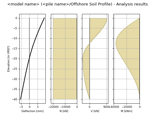
Example

The plot looks like:

plot_forces(assign=False)[source]

Plots the pile sectional forces.

Parameters:: assign (bool, optional) – by default False
Returns:: if assign is True, a matplotlib figure is returned
Return type:: None or matplotlib.pyplot.figure

Example

The plot looks like:

plot_lateral_results(assign=False)[source]

Plots the pile deflection and sectional forces.

Parameters:: assign (bool, optional) – by default False
Returns:: if assign is True, a matplotlib figure is returned
Return type:: None or matplotlib.pyplot.figure

Example

The plot looks like:

plot_axial_results(assign=False)[source]

Plots the pile settlements and normal forces.

Parameters:: assign (bool, optional) – by default False
Returns:: if assign is True, a matplotlib figure is returned
Return type:: None or matplotlib.pyplot.figure

plot(assign=False)[source]

Same behaviour as openpile.analyze.plot_lateral_results().

Parameters:: assign (bool, optional) – by default False
Returns:: if assign is True, a matplotlib figure is returned
Return type:: None or matplotlib.pyplot.figure

Example

The plot looks like:

details()[source]

Provide a summary of the results.

Returns:: info on the results
Return type:: dict

openpile.winkler.beam(model)[source]

Function where loading or displacement defined in the model boundary conditions are used to solve the system of equations, this is a linear problem and is solved with one iteration.

Parameters:: model (openpile.construct.Model object) – Model where structure and boundary conditions are defined.
Returns:: results – Results of the analysis
Return type:: openpile.compute.Result object

openpile.winkler.winkler(model, max_iter=100)[source]

Function where loading or displacement defined in the model boundary conditions are used to solve the system of equations via the iterative Newton-Raphson scheme.

Parameters:

model (openpile.construct.Model object) – Model where structure and boundary conditions are defined.
max_iter (int, by defaut 100) – maximum number of iterations for convergence

Returns:

results – Results of the analysis

Return type:

openpile.analyses.Result object

py_curves module 

openpile.utils.py_curves.bothkennar_clay(X, Su, G0, D, output_length=20)[source]

Creates a spring from the PISA clay formulation published by Burd et al 2020 (see [BABH20]) and calibrated based on Bothkennar clay response (a normally consolidated soft clay).

Parameters:

X (float) – Depth below ground level [unit: m]
Su (float) – Undrained shear strength [unit: kPa]
G0 (float) – Small-strain shear modulus [unit: kPa]
D (float) – Pile diameter [unit: m]
output_length (int, optional) – Number of datapoints in the curve, by default 20

Returns:

1darray – y vector [unit: m]
1darray – p vector [unit: kN/m]

See also

openpile.utils.py_curves.cowden_clay(), openpile.utils.py_curves.custom_clay()

openpile.utils.py_curves.cowden_clay(X, Su, G0, D, output_length=20)[source]

Creates a spring from the PISA clay formulation published by Byrne et al 2020 (see [BHBG20]) and calibrated based pile load tests at Cowden (north east coast of England).

Parameters:

X (float) – Depth below ground level [unit: m]
Su (float) – Undrained shear strength [unit: kPa]
G0 (float) – Small-strain shear modulus [unit: kPa]
D (float) – Pile diameter [unit: m]
output_length (int, optional) – Number of datapoints in the curve, by default 20

Returns:

1darray – y vector [unit: m]
1darray – p vector [unit: kN/m]

See also

openpile.utils.py_curves.bothkennar_clay(), openpile.utils.py_curves.custom_clay()

openpile.utils.py_curves.dunkirk_sand(sig, X, Dr, G0, D, L, output_length=20)[source]

Creates a lateral spring from the PISA sand formulation published by Burd et al (2020) (see [BTZA20]). Also called the General Dunkirk Sand Model (GDSM).

Parameters:

sig (float) – vertical/overburden effective stress [unit: kPa]
X (float) – Depth below ground level [unit: m]
Dr (float) – Sand relative density Value must be between 0 and 100 [unit: -]
G0 (float) – Small-strain shear modulus [unit: kPa]
D (float) – Pile diameter [unit: m]
L (float) – Embedded pile length [unit: m]
output_length (int, optional) – Number of datapoints in the curve, by default 20

Returns:

1darray – y vector [unit: m]
1darray – p vector [unit: kN/m]

Notes

The curve backbone is defined as a conic function, see below.

_images/PISA_conic_function.png — Fig. 4 PISA Conic function: (a) conic form; (b) bilinear form, after [BHBG20].

openpile.utils.py_curves.api_sand(sig, X, phi, D, kind='static', below_water_table=True, k=0.0, ymax=0.0, output_length=20)[source]

Creates the API sand p-y curve from relevant input.

Parameters:

sig (float) – Vertical effective stress [unit: kPa]
X (float) – Depth of the curve w.r.t. mudline [unit: m]
phi (float) – internal angle of friction of the sand layer [unit: degrees]
D (float) – Pile width [unit: m]
kind (str, by default "static") – types of curves, can be of (“static”,”cyclic”)
below_water_table (bool, by default False) – switch to calculate initial subgrade modulus below/above water table
k (float, by default 0.0) – user-defined initial subgrade modulus [kN/m^3], if kept as zero, it is calculated as per API guidelines, see Notes below
ymax (float, by default 0.0) – maximum value of y, default goes to 99.9% of ultimate resistance
output_length (int, by default 20) – Number of discrete point along the springs, cannot be less than 8

Returns:

1darray – y vector [unit: m]
1darray – p vector [unit: kN/m]

Notes

p-y formulation

The API sand p-y formulation is presented in both the API and DNVGL standards, see, [DNV-RP-C212], [API2000] or [API2014].

Granular soils are modelled by the sand p-y model as described with the following backbone formula:

\[p = A \cdot P_{max} \cdot \tanh \left( \frac{k \cdot X}{A \cdot P_{max} } y \right)\]

where:

\(A\) is a factor to account for static of cyclic loading
\(P_{max}\) is the ultimate resistance of the p-y curve
\(k\) is the initial modulus of subgrade reaction
\(X\) is the depth below mudline of the p-y curve.

Factor A

The factor A takes into account whether the curve represent static(also called monotonic) or cycling loading and is equal to:

\[\begin{split}A = \begin{cases} \begin{split} 0.9 & \text{ for cyclic loading} \\ \\ 3 - 0.8 \frac{X}{D} \ge 0.9 & \text{ for static loading} \end{split} \end{cases}\end{split}\]

where:

\(D\) is the pile diameter.

Initial subgrade reaction modulus

The initial subgrade reaction, represented by the factor k is approximated by the following equation in which the output is given in kN/m³ and where \(\phi\) is inserted in degrees:

\[\begin{split}k = \begin{cases} \begin{split} 197.8 \cdot \phi^2 - 10232 \cdot \phi + 136820 \ge 5400 & \text{ , below water table} \\ \\ 215.3 \cdot \phi^2 - 8232 \cdot \phi + 63657 \ge 5400 & \text{ , above water table} \end{split} \end{cases}\end{split}\]

The equation is a fit to the recommended values in [API2000]. The correspondence of this fit is illustrated in below figure:

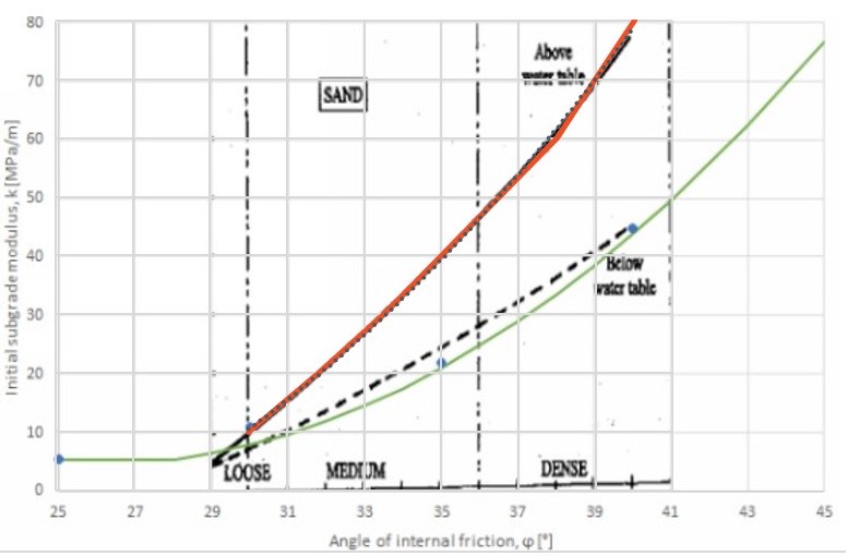
_images/k_vs_phi.jpg — Fig. 5 Subgrade reaction moduli fits calculated by openpile.

Note

The initial subgrade modulus can be user-defined by setting the parameter ‘k’ to a value greater than zero. Furthermore, many researchers have proposed different values for the initial subgrade modulus, see openpile.soilmodels.hooks.InitialSubgradeReaction.

Ultimate resistance

The ultimate resistance \(P_{max}\) is calculated via the coefficients C1, C2 and C3 found in the below figure.

_images/C_coeffs_graph.jpg — Fig. 6 Coefficients to calculate the maximum resistance. (as given in [MuOn84])

The ultimate resistance is found via the below equation:

\[P_{max} = \left( C1 \cdot \sigma^{\prime} \cdot X + C2 \cdot \sigma^{\prime} \cdot D \right) \lt C3 \cdot \sigma^{\prime} \cdot D\]

where:

\(\sigma^{\prime}\) is the vertical effective stress

openpile.utils.py_curves.api_clay(sig, X, Su, eps50, D, J=0.5, kind='static', ymax=0.0, output_length=20)[source]

Creates the API clay p-y curve from API RP2GEO (2014) from relevant input.

Parameters:

sig (float) – Vertical effective stress [unit: kPa]
X (float) – Depth of the curve w.r.t. mudline [unit: m]
Su (float) – Undrained shear strength [unit: kPa]
eps50 (float) – strain at 50% ultimate resistance [-]
D (float) – Pile width [unit: m]
J (float, by default 0.5) – empirical factor varying depending on clay stiffness
kind (str, by default "static") – types of curves, can be of (“static”,”cyclic”)
ymax (float, by default 0.0) – maximum value of y, if null the maximum is calculated such that the whole curve is computed
output_length (int, by default 20) – Number of discrete point along the springs, cannot be less than 8

Returns:

1darray – y vector [unit: m]
1darray – p vector [unit: kN/m]

Notes

The p-y clay formulation is presented in both the API and DNVGL standards, see [DNV-RP-C212] and [API2014].

The p-y curve is defined as per Matlock original equations (see notes in openpile.utils.py_curves.matlock_1970()) but defined at specific points, in a piece-wise manner.

Static piece-wise points are defined as follows:

\(p/P_{max}\)	\(y/y_{50}\)
0.00	0.0
0.23	0.1
0.33	0.3
0.50	1.0
0.72	3
1.00	8
1.00	\(\infty\)

Cyclic piece-wise points are defined as follows:

\(p/P_{max}\)	\(y/y_{50}\)
0.00	0.0
0.23	0.1
0.33	0.3
0.50	1.0
0.72	3.0
\(\min\left(0.72; 0.72 \dfrac{z}{X_R}\right)\)	15.0
\(\min\left(0.72; 0.72 \dfrac{z}{X_R}\right)\)	\(\infty\)

where:

\(z\) is the depth below mudline
\(X_R\) is the transition zone depth below mudline
\(y_{50}\) is the equivalent displacement for deformation at 50% ultimate resistance
\(P_{max}\) is the ultimate resistance of the p-y curve

openpile.utils.py_curves.matlock_1970(sig, X, Su, eps50, D, J=0.5, kind='static', ymax=0.0, output_length=20)[source]

Creates the original clay p-y curve from the work performed by [Matl70].

Parameters:

sig (float) – Vertical effective stress [unit: kPa]
X (float) – Depth of the curve w.r.t. mudline [unit: m]
Su (float) – Undrained shear strength [unit: kPa]
eps50 (float) – strain at 50% ultimate resistance [-]
D (float) – Pile width [unit: m]
J (float, by default 0.5) – empirical factor varying depending on clay stiffness
kind (str, by default "static") – types of curves, can be of (“static”,”cyclic”)
ymax (float, by default 0.0) – maximum value of y, if null the maximum is calculated such that the whole curve is computed
output_length (int, by default 20) – Number of discrete point along the springs, cannot be less than 9

Returns:

1darray – y vector [unit: m]
1darray – p vector [unit: kN/m]

Notes

Ultimate resistance

The ultimate resistance is calculated via the capacity of two failure mechanisms, one that is shallow (wedge-type failure) and another that is deep (flow-around failure).

\[\begin{split}P_{max} &= min(P_{shallow}, P_{deep}) \\\\ P_{shallow} &= D (3 S_u + \sigma^{\prime}) + J \cdot S_u \cdot X \\\\ P_{deep} &= 9 \cdot S_u \cdot D\end{split}\]

where:

\(S_u\) is the undrained shear strßength in Unconfined and unconsolidated (UU) Trixial tests.
\(\sigma^{\prime}\) is the vertical effective stress.
\(J\) is an empirical factor determined by Matlock to fit results to pile load tests. This value can vary from 0.25 to 0.50 depending on the clay characteristics
\(X\) is the depth below ground level

Strain normalization

Strain normalization is performed with a parameter \(y_{50}\) that is used to scale the curve with respect to the structure’s scale and soil type.

\[y_{50} = 2.5 \cdot \varepsilon_{50} \cdot D\]

where:

\(D\) is the pile width or diameter
\(\varepsilon_{50}\) is the strain at 50% ultimate resistance in Unconfined and unconsolidated (UU) Triaxial tests.

Transition zone

A transition zone is defined which corresponds to the depth at which the failure around the pile is not governed by the free-field boundary, i.e. the ground level. Below the transition zone, a flow-around type of failure.

The transition zone is defined by the following formula:

\[X_R = \left( \frac{6 \cdot D}{\gamma^{\prime} \cdot \frac{D}{S_u} + J} \right) \ge 2.5 \cdot D\]

Initial stiffness of p-y curve

The initial stiffness \(k_{ini}\) is infinite and can be capped from the Matlock original as in openpile.utils.py_curves.api_clay():

p-y formulation (static loading, Neq = 1)

\[\begin{split}p = \begin{cases} \begin{split} 0.5 \cdot P_{max} \left( \frac{y}{y_{50}} \right)^{0.33} & \text{ for } y \le 8 y_{50} \\ \\ P_{max} & \text{ for } y \gt 8 y_{50} \end{split} \end{cases}\end{split}\]

p-y formulation (cyclic loading, Neq > 1)

\[\begin{split}p = \begin{cases} \begin{split} 0.5 \cdot P_{max} \left( \frac{y}{y_{50}} \right)^{0.33} & \text{ for } y \le 3 y_{50} \\ \\ 0.72 \cdot P_{max} & \text{ for } y \gt 3 y_{50} \end{split} \end{cases}\end{split}\]

For cyclic loading and curves above the transition zone ( i.e. \(X \le Xr\)), the p-y curve can be generated according to:

\[\begin{split}p = \begin{cases} \begin{split} 0.5 \cdot P_{max} \left( \frac{y}{y_{50}} \right) & \text{ for } y \le 3 y_{50} \\ \\ 0.72 \cdot P_{max} \left[ 1 - \left( 1 - \frac{X}{X_R} \right) \left( \frac{y - 3 y_{50}}{12 y_{50}} \right) \right] & \text{ for } 3 y_{50} \lt y \le 15 y_{50} \\ \\ 0.72 \cdot P_{max} \left( \frac{X}{X_R} \right) & \text{ for } y \gt 15 y_{50} \\ \end{split} \end{cases}\end{split}\]

openpile.utils.py_curves.modified_Matlock(sig, X, Su, eps50, D, J=0.5, kind='cyclic', ymax=0.0, output_length=20)[source]

Creates the Modified Matlock for stiff clay p-y curve as defined in Bathacharya et al 2006 (see [BaCA06]).

The modification takes places in the cyclic version of the curves. Static curves are kept the same as the original curves (see [Matl70]), see Openpile.utils.py_curves.matlock_1970().

Parameters:

sig (float) – Vertical effective stress [unit: kPa]
X (float) – Depth of the curve w.r.t. mudline [unit: m]
Su (float) – Undrained shear strength [unit: kPa]
eps50 (float) – strain at 50% ultimate resistance [-]
D (float) – Pile width [unit: m]
J (float, by default 0.5) – empirical factor varying depending on clay stiffness
kind (str, by default "cyclic") – types of curves, can be of (“static”,”cyclic”)
ymax (float, by default 0.0) – maximum value of y, if null the maximum is calculated such that the whole curve is computed
output_length (int, by default 20) – Number of discrete point along the springs, cannot be less than 8

Returns:

1darray – y vector [unit: m]
1darray – p vector [unit: kN/m]

Notes

Differences with standard Matlock (1970) formula: For an undrained shear strength of 96 kPa (assumed as the threshold at which a clay is considered stiff), this formulation may be deemed more relevant to account for a more brittle fracture and degradation of the soil, see [BaCA06].

Fig. 7 Schematic of original (soft clay response) and modified (stiff clay response), after [BaCA06].

openpile.utils.py_curves.reese_weakrock(Ei, qu, RQD, xr, D, k=0.0005, output_length=20)[source]

creates the Reese weakrock p-y curve based on the work of Reese (1997), see reference [Rees97].

Parameters:

Ei (float) – initial rock mass modulus of rock [kPa]
qu (float) – unconfined compressive strength of rock [kPa]
RQD (float) – Rock Quality Designation [%]
xr (float) – depth from rock surface [m]
D (float) – pile width [m]
k (float, optional) – dimensional constant, randing from 0.0005 to 0.00005, by default 0.0005
output_length (int, optional) – length of output arrays, by default 20, cannot be less than 8

Returns:

1darray – y vector [unit: m]
1darray – p vector [unit: kN/m]

Notes

This formulation was derived for weak rocks and based on [Rees97]. This empirical model is mostly based on experimental data of pile load tests near San Francisco where the rock unconfined compressive strength varies from 1.86 MPa near the surface to 16.0 MPa. Pressuremeter tests results were used by Reese in this formulation as the initial modulus of the rock.

The curve is characterized by a linear initial portion, a non-linear response for the remaining part of the curve, and a maximum resistance value that can be mobilized

Ultimate resistance of rock

\[P_{max} = \alpha \cdot q_u \cdot D \left(1 + 1.4 \dfrac{x_r}{D}\right) \le 5.2 \alpha \cdot q_u \cdot D\]

where:

\(\alpha = 1 - \dfrac{2}{3} \dfrac{\text{RQD}}{100}\)
\(\text{RQD}\) is the rock quality designation in percentage
\(q_u\) is the unconfined compressive strength of rock
\(D\) is the pile diameter
\(x_r\) is the depth from rock surface

Initial portion of p-y curve

The initial part of the curve is defined for \(y \le yA\), with a linear p-y curve stiffness of \(E_{py_i}\).

\[\begin{split}y_A &= \left(\dfrac{P_{max}}{2 \cdot y_{rm}^{0.25} \cdot E_{py_i}}\right)^{4/3} \\ \\ E_{py_i} &= \left(100 + 400 \dfrac{x_r}{3D} \right) E_i \le 500 E_i\end{split}\]

where:

\(E_rm\) is the rock mass modulus of rock
\(y_{rm} = k \cdot D\)
\(k\) is a dimensional constant ranging from 0.0005 to 0.00005

Remaining non-linear response

The remaining portion of the curve is defined with the following equation:

\[p = \dfrac{P_{max}}{2} \left(\dfrac{y}{y_{rm}}\right)^{1/4} \le P_{max}\]

openpile.utils.py_curves.custom_pisa_sand(sig, G0, D, X_ult, n, k, Y_ult, output_length=20)[source]

Creates a lateral spring with the PISA sand formulation and custom user inputs.

Parameters:

sig (float) – vertical/overburden effective stress [unit: kPa]
G0 (float) – Small-strain shear modulus [unit: kPa]
X_ult (float) – Normalized displacement at maximum strength
k (float) – Normalized stiffness parameter
n (float) – Normalized curvature parameter, must be between 0 and 1
Y_ult (float) – Normalized maximum strength parameter
output_length (int, optional) – Number of datapoints in the curve, by default 20
D (float) –

Returns:

1darray – y vector [unit: m]
1darray – p vector [unit: kN/m]

See also

openpile.utils.py_curves.dunkirk_sand(), openpile.utils.hooks.dunkirk_sand_pisa_norm_param()

Example

import matplotlib.pyplot as plt
from openpile.utils.py_curves import custom_pisa_sand, dunkirk_sand

openpile.utils.py_curves.custom_pisa_clay(Su, G0, D, X_ult, n, k, Y_ult, output_length=20)[source]

Creates a spring from the PISA clay formulation published by Byrne et al 2020 (see [BHBG20]) and calibrated based pile load tests at Cowden (north east coast of England).

Parameters:

Su (float) – Undrained shear strength [unit: kPa]
G0 (float) – Small-strain shear modulus [unit: kPa]
D (float) – Pile diameter [unit: m]
X_ult (float) – Normalized displacement at maximum strength
k (float) – Normalized stiffness parameter
n (float) – Normalized curvature parameter, must be between 0 and 1
Y_ult (float) – Normalized maximum strength parameter
output_length (int, optional) – Number of datapoints in the curve, by default 20

Returns:

1darray – y vector [unit: m]
1darray – p vector [unit: kN/m]

See also

openpile.utils.py_curves.cowden_clay(), openpile.utils.py_curves.bothkennar_clay(), openpile.utils.hooks.cowden_clay_pisa_norm_param()

mt_curves module 

openpile.utils.mt_curves.bothkennar_clay(X, Su, G0, D, output_length=20)[source]

Create the rotational springs from the PISA clay formulation published by Burd et al 2020 (see [BABH20]) and calibrated based on Bothkennar clay response (a normally consolidated soft clay).

Parameters:

X (float) – Depth below ground level [unit: m]
Su (float) – Undrained shear strength [unit: kPa]
G0 (float) – Small-strain shear modulus [unit: kPa]
D (float) – Pile diameter [unit: m]
output_length (int, optional) – Number of datapoints in the curve, by default 20

Returns:

1darray – t vector of length [unit: rad]
1darray – m vector [unit: kN]

openpile.utils.mt_curves.cowden_clay(X, Su, G0, D, output_length=20)[source]

Create the rotational springs from the PISA clay formulation published by Byrne et al 2020 (see [BHBG20]) and calibrated based pile load tests at Cowden (north east coast of England).

Parameters:

X (float) – Depth below ground level [unit: m]
Su (float) – Undrained shear strength [unit: kPa]
G0 (float) – Small-strain shear modulus [unit: kPa]
D (float) – Pile diameter [unit: m]
output_length (int, optional) – Number of datapoints in the curve, by default 20

Returns:

1darray – t vector of length [unit: rad]
1darray – m vector [unit: kN]

openpile.utils.mt_curves.dunkirk_sand(sig, X, Dr, G0, p, D, L, output_length=20)[source]

Create the rotational springs from the PISA sand formulation published by Burd et al (2020) (see [BTZA20]). Also called the General Dunkirk Sand Model (GDSM)

Parameters:

sig (float) – vertical/overburden effective stress [unit: kPa]
X (float) – Depth below ground level [unit: m]
Dr (float) – Sand relative density Value must be between 0 and 100 [unit: -]
G0 (float) – Small-strain shear modulus [unit: kPa]
p (float) – radial stress computed via p-y curves [unit: kN/m]
D (float) – Pile diameter [unit: m]
L (float) – Embedded pile length [unit: m]
output_length (int, optional) – Number of datapoints in the curve, by default 20

Returns:

1darray – t vector of length [unit: rad]
1darray – m vector [unit: kN]

openpile.utils.mt_curves.custom_pisa_sand(sig, G0, p, D, X_ult, n, k, Y_ult, output_length=20)[source]

Creates a rotational spring with the PISA sand formulation and custom user inputs.

Parameters:

sig (float) – vertical/overburden effective stress [unit: kPa]
G0 (float) – Small-strain shear modulus [unit: kPa]
p (float) – Radial stress computed via p-y curves [unit: kN/m]
D (float) – Pile diameter [m]
X_ult (float) – Normalized displacement at maximum strength
k (float) – Normalized stiffness parameter
n (float) – Normalized curvature parameter, must be between 0 and 1
Y_ult (float) – Normalized maximum strength parameter
output_length (int, optional) – Number of datapoints in the curve, by default 20

Returns:

1darray – y vector [unit: m]
1darray – p vector [unit: kN/m]

openpile.utils.mt_curves.custom_pisa_clay(Su, G0, D, X_ult, n, k, Y_ult, output_length=20)[source]

Creates a rotational spring with the PISA clay formulation and custom user inputs.

Parameters:

Su (float) – Undrained shear strength [unit: kPa]
G0 (float) – Small-strain shear modulus [unit: kPa]
D (float) – Pile diameter [unit: m]
X_ult (float) – Normalized displacement at maximum strength
k (float) – Normalized stiffness parameter
n (float) – Normalized curvature parameter, must be between 0 and 1
Y_ult (float) – Normalized maximum strength parameter
output_length (int, optional) – Number of datapoints in the curve, by default 20

Returns:

1darray – y vector [unit: m]
1darray – p vector [unit: kN/m]

tz_curves module 

openpile.utils.tz_curves.backbone_api_clay(residual=0.9, tensile_factor=1.0, output_length=15)[source]

Creates the API clay t-z curve backbone (i.e. normalized with strength and diameter) from relevant input as per [API2000].

Parameters:

D (float) – Pile width [unit: m]
residual (float) – residual strength after peak strength, according to API-RP-2A, this value is between 0.7 and 0.9, default to 0.9
tensile_factor (float) – strength factor for negative values of the curve
output_length (int, optional) – Number of discrete point along the springs, cannot be lower than 15, by default 15

Returns:

numpy 1darray – t vector [unit: kPa]
numpy 1darray – z vector [unit: m]

openpile.utils.tz_curves.api_clay(sig, Su, D, alpha_limit=1.0, residual=0.9, tensile_factor=1.0, output_length=15)[source]

Creates the API clay t-z curve from relevant input as per [API2000].

Parameters:

sig (float) – Vertical effective stress [unit: kPa]
Su (float) – Undrained shear strength [unit: kPa]
D (float) – Pile width [unit: m]
alpha_limit (float) – maximum value of the alpha parameter, default to 1.0
residual (float) – residual strength after peak strength, according to API-RP-2A, this value is between 0.7 and 0.9, default to 0.9
tensile_factor (float) – strength factor for negative values of the curve
output_length (int, optional) – Number of discrete point along the springs, cannot be lower than 15, by default 15

Returns:

numpy 1darray – t vector [unit: kPa]
numpy 1darray – z vector [unit: m]

Notes

The backbone curve is computed via the piecewise formulation by [API2000] or through Kraft’s formulation that captures small-strain characteristics of the soil [KrRK81] in the backbone curve.

Note

Kraft’s formulation is accessed by the user by stipulating the small-strain shear stiffness of the soil, \(G_0\)

The API guidelines describe the axial soil springs in a manner that accounts for the undrained shear strength of the clay. The springs are characterized as follows:

Unit Skin Friction \(f_s\): For clay, this is based on the undrained shear strength \(S_u\) of the soil and a factor that accounts for the adhesion between the clay and the pile.
\[f_s = \alpha \cdot S_u < f_{s,\text{max}}\]

where:
- \(\alpha\) is the adhesion factor, which depends on the type of clay and the pile material. It typically ranges from 0.5 to 1.0 for soft clays and 0.3 to 0.6 for stiff clays. As per the API guidelines, this adhesion factor can be calculated as:
- \(S_u\) is the undrained shear strength of the clay.
- Limit Skin Friction \(f_{s,\text{max}}\) is the maximum unit skin friction for clay, which can be directly related to the undrained shear strength and the adhesion factor. In general, the limit skin friction is set to the undrained shear strength.
A backbone curve computed via the piecewise formulation seen in [API2000].

openpile.utils.tz_curves.api_clay_kraft(sig, Su, D, G0, alpha_limit=1.0, residual=1.0, tensile_factor=1.0, RF=0.9, zif=10.0, output_length=15)[source]

Creates the API clay t-z curve (see [API2000]) with the Kraft et al (1981) formulation (see [KrRK81]).

Parameters:

sig (float) – Vertical effective stress [unit: kPa]
Su (float) – Undrained shear strength [unit: kPa]
D (float) – Pile diameter [unit: m]
G0 (float) – small-strain stiffness [unit: kPa]
alpha_limit (float) – limit of the alpha parameter, by default 1.0
residual (float) – residual strength after peak strength, by default 1.0
tensile_factor (float) – strength factor for negative values of the curve, by default 1.0
RF (float) – curve fitting factor as per Kraft et al. (1981), by default 0.9
zif (float) – dimensionless zone of influence as per Kraft et al (1981) that corresponds to the radius of the zone of influence divided by the pile radius, by default 10.0
output_length (int, optional) – Number of discrete point along the springs, cannot be lower than 15, by default 15

Returns:

numpy 1darray – t vector [unit: kPa]
numpy 1darray – z vector [unit: m]

See also

openpile.utils.tz_curves.api_clay()

Notes

The backbone curve is computed via the piecewise formulation by [API2000] or through Kraft’s formulation that captures small-strain characteristics of the soil [KrRK81] in the backbone curve.

Note

Kraft’s formulation is accessed by the user by stipulating the small-strain shear stiffness of the soil, \(G_0\)

For clay, the API guidelines describe the axial soil springs in a manner that accounts for the undrained shear strength of the clay. The springs are characterized as follows:

Unit Skin Friction \(f_s\): For clay, this is based on the undrained shear strength \(S_u\) of the soil and a factor that accounts for the adhesion between the clay and the pile.
\[f_s = \alpha \cdot S_u < f_{s,\text{max}}\]

where:
- \(\alpha\) is the adhesion factor, which depends on the type of clay and the pile material. It typically ranges from 0.5 to 1.0 for soft clays and 0.3 to 0.6 for stiff clays. As per the API guidelines, this adhesion factor can be calculated as:
- \(S_u\) is the undrained shear strength of the clay.
- Limit Skin Friction \(f_{s,\text{max}}\) is the maximum unit skin friction for clay, which can be directly related to the undrained shear strength and the adhesion factor. In general, the limit skin friction is set to the undrained shear strength.
A backbone curve computed via the piecewise formulation seen in [API2000].

openpile.utils.tz_curves.backbone_api_sand(tensile_factor=1.0, output_length=7)[source]

Creates the API sand t-z curve (see [API2000]).

Parameters:

tensile_factor (float) – strength factor for negative values of the curve
output_length (int, optional) – Number of discrete point along the springs, cannot be lower than 7, by default 7

Returns:

numpy 1darray – t vector [unit: kPa]
numpy 1darray – z vector [unit: m]

openpile.utils.tz_curves.api_sand(sig, delta, K=0.8, tensile_factor=1.0, output_length=7)[source]

Creates the API sand t-z curve (see [API2000]).

Parameters:

sig (float) – Vertical effective stress [unit: kPa]
delta (float) – interface friction angle [unit: degrees]
K (float) – coefficient of lateral pressure (0.8 for open-ended piles and 1.0 for cloased-ended)
tensile_factor (float) – strength factor for negative values of the curve
output_length (int, optional) – Number of discrete point along the springs, cannot be lower than 7, by default 7

Returns:

numpy 1darray – t vector [unit: kPa]
numpy 1darray – z vector [unit: m]

Notes

The backbone curve is computed via the piecewise formulation by [API2000] or through Kraft’s formulation that captures small-strain characteristics of the soil [KrRK81] in the backbone curve.

Note

Kraft’s formulation is accessed by the user by stipulating the small-strain shear stiffness of the soil, \(G_0\)

The API guidelines provide methods to estimate the resistance offered by sandy soils along the pile. These springs are defined based on the following considerations:

Unit Skin Friction \(f_s\): This is the frictional resistance per unit area along the pile shaft. It depends on the effective overburden pressure and the soil-pile interface properties.
\[\]

f_s = sigma_v^prime cdot K cdot tan(delta) < f_{s,text{max}}

where:
- sigma_v^prime is the effective vertical stress at the depth considered.
- K is the coefficient of horizontal earth pressure (typically ranges from 0.4 to 1.0 for sands).
- delta is the angle of friction between the pile and the sand, often taken as a fraction of the soil’s internal friction angle \(\varphi\) (usually \(\delta = 0.7 \varphi\) to \(\varphi\)).
- Limit Skin Friction \(f_{s,\text{max}}\) is the maximum unit skin friction that can be mobilized. It is typically given by empirical correlations or laboratory tests. The following is assumed in OpenPile:
Table 1 Correlation between interface friction angle and shaft friction

\(\delta\) [degrees]

15

20

25

30

35

\(f_{s,\texttt{max}}\) [kPa]

47.8

67

81.3

95.7

114.8
A backbone curve computed via the piecewise formulation seen in [API2000].

openpile.utils.tz_curves.api_sand_kraft(sig, delta, D, G0, K=0.8, residual=1.0, tensile_factor=1.0, RF=0.9, zif=10.0, output_length=15)[source]

Creates the API sand t-z curve (see [API2000]) with the Kraft et al (1981) formulation (see [KrRK81]).

Parameters:

sig (float) – Vertical effective stress [unit: kPa]
delta (float) – interface friction angle [unit: degrees]
D (float) – Pile width [unit: m]
G0 (float) – small-strain stiffness [unit: kPa]
K (float) – coefficient of lateral pressure (0.8 for open-ended piles and 1.0 for cloased-ended), by default 0.8
residual (float) – residual strength after peak strength, by default 1.0
tensile_factor (float) – strength factor for negative values of the curve, by default 1.0
RF (float) – curve fitting factor as per Kraft et al. (1981), by default 0.9
zif (float) – dimensionless zone of influence as per Kraft et al (1981) that corresponds to the radius of the zone of influence divided by the pile radius, by default 10.0
output_length (int, optional) – Number of discrete point along the springs, cannot be lower than 15, by default 15

Returns:

numpy 1darray – t vector [unit: kPa]
numpy 1darray – z vector [unit: m]

See also

openpile.utils.tz_curves.api_sand()

Notes

The backbone curve is computed via the piecewise formulation by [API2000] or through Kraft’s formulation that captures small-strain characteristics of the soil [KrRK81] in the backbone curve.

Note

Kraft’s formulation is accessed by the user by stipulating the small-strain shear stiffness of the soil, \(G_0\)

The API guidelines provide methods to estimate the resistance offered by sandy soils along the pile. These springs are defined based on the following considerations:

Unit Skin Friction \(f_s\): This is the frictional resistance per unit area along the pile shaft. It depends on the effective overburden pressure and the soil-pile interface properties.
\[\]

f_s = sigma_v^prime cdot K cdot tan(delta) < f_{s,text{max}}

where:
- sigma_v^prime is the effective vertical stress at the depth considered.
- K is the coefficient of horizontal earth pressure (typically ranges from 0.4 to 1.0 for sands).
- delta is the angle of friction between the pile and the sand, often taken as a fraction of the soil’s internal friction angle \(\varphi\) (usually \(\delta = 0.7 \varphi\) to \(\varphi\)).
- Limit Skin Friction \(f_{s,\text{max}}\) is the maximum unit skin friction that can be mobilized. It is typically given by empirical correlations or laboratory tests. The following is assumed in OpenPile:
Table 2 Correlation between interface friction angle and shaft friction

\(\delta\) [degrees]

15

20

25

30

35

\(f_{s,\texttt{max}}\) [kPa]

47.8

67

81.3

95.7

114.8
A backbone curve computed via the piecewise formulation seen in [API2000].

qz_curves module 

openpile.utils.qz_curves.api_clay(Su, D, output_length=15)[source]

Creates the API clay Q.z curve from relevant input.

Parameters:

Su (float) – Undrained shear strength [unit: kPa]
D (float) – Pile diameter [unit: m]
output_length (int, optional) – Number of discrete point along the springs, cannot be lower than 15, by default 15

Returns:

numpy 1darray – z vector [unit: m]
numpy 1darray – Q vector [unit: kPa]

Notes

The maximum resistance is calculated as follows:

API clay: \(Q_{max} = 9 S_u\)

where \(S_u\) is the clay undrained shear strength.

The backbone curve is computed via the piecewise formulation presented in [API2000].

openpile.utils.qz_curves.api_sand(sig, delta, D, output_length=15)[source]

Creates the API sand Q.z curve from relevant input.

Parameters:

sig (float) – Vertical effective stress [unit: kPa]
delta (float) – interface friction angle [unit: degrees]
D (float) – Pile diameter [unit: m]
output_length (int, optional) – Number of discrete point along the springs, cannot be lower than 15, by default 15

Returns:

numpy 1darray – z vector [unit: m]
numpy 1darray – Q vector [unit: kPa]

Notes

The maximum resistance is calculated as follows:

API sand: \(Q_{max} = N_q \sigma^\prime_v\)

where \(\sigma_v^\prime\) is the overburden effective stress and \(N_q\) is the end-bearing factor depending on the interface friction angle \(\varphi\), see below table.

\(\varphi\) [degrees]	15.0	20.0	25.0	30.0	35.0
\(N_q\) [kPa]	8.0	12.0	20.0	40.0	50.0
\(Q_{max}\) [kPa]	1900	2900	4800	9600	12000

The backbone curve is computed via the piecewise formulation presented in [API2000].

hooks module 

openpile.utils.hooks.durkhop(D, ra=0.3)[source]

This function generates p-multipliers as per Durkhop et al (see [Duhr09]) for application to cyclic curves of the openpile.soilmodels.API_sand model.

The default behaviour, i.e. when the parameter ra = 0.3 is that the API sand cyclic curves are unchanged with a equivalent number of cycles equal to 100. When the parameter ra is equal to 1.0, the cyclic curves are approach the static curves. In between 0.3 and 1.0, the multipliers may be thought as cyclic curves with a lower number of equivalent cycles.

Parameters:

D (float) – Pile diameter [m]
ra (float, optional) – empirical factor dependent on the number of load cycles, 1.0 for monotonic loading and 0.3 for cyclic loading at 100 cycles, by default 0.3

Returns:

callable for use as p_multipler in openpile.soilmodels.API_sand in cyclic mode.

Return type:

object

Example

import matplotlib.pyplot as plt
from openpile.construct import Layer
from openpile.utils import hooks
from openpile.soilmodels import API_sand
# settings for py curve generation
kw = {'sig':50, 'X':5, 'layer_height':10, 'depth_from_top_of_layer':5, 'D':5, 'L':30}
# a, b soil models are traditional cyclic and static API sand models
a = API_sand(
    phi=33,
    kind="static",
)
b = API_sand(
    phi=33,
    kind="cyclic",
)
plt.plot(*a.py_spring_fct(**kw), label='static')
plt.plot(*b.py_spring_fct(**kw), label='cyclic')
# soil model c is the API sand model with `durkhop` multipliers
for ra in [0.3,0.45,0.6,0.75,0.9]:
    c = API_sand(
        phi=33,
        kind="cyclic",
        p_multiplier=hooks.durkhop(D=7.0, ra=ra)
    )
    plt.plot(*c.py_spring_fct(**kw), ':',label=f'Durkhop multipliers, ra={ra}')
plt.legend()

Reference

[Duhr09]

Dührkop, J. (2009). Zum Einfluss von Aufweitungen und zyklischen Lasten auf das Verformungsverhalten lateral 385 beanspruchter Pfähle in Sand. Ph.D. Thesis, Institut für Geotechnik und Baubetrieb, Technische Universität Hamburg-Harburg, Vol. 20 (in German).

openpile.utils.hooks.durkhop_normalized(D, ra=0.3)[source]

This function generates multipliers that represent ratios the cyclic and monotonic curves of the traditional API sand model.

Parameters:

D (float) – Pile diameter [m]
ra (float, optional) – empirical factor dependent on the number of load cycles, 1.0 for monotonic loading and 0.3 for cyclic loading at 100 cycles, by default 0.3

Returns:

callable for use as p_multipler in openpile.soilmodels.LateralModel or openpile.soilmodels.AxialModel The function input is the depth and the function output is the multiplier applied for the spring at the said depth.

Return type:

object

Example

See also

None

class openpile.utils.hooks.PISA_depth_variation[source]

Bases: object

stores functions that returns the depth varying normalized parameters of the p-y, m-t, H-b and M-b conic formulations as per [BTZA20] and [BHBG20], and [BABH20].

These functions can be then be used to model the original models, e.g. Cowden Clay, or make modifications to the original models.

Example

import matplotlib.pyplot as plt
from openpile.utils.py_curves import custom_pisa_sand, dunkirk_sand
from openpile.utils.hooks import PISA_depth_variation

# plot original dunkirk sand curve
params = {'sig':50, 'X':5, 'Dr':75, 'G0':50e3, 'D':6, 'L':20}
plt.plot(*dunkirk_sand(**params), label='Original Dunkirk Sand model', linestyle='-')

# load PISA dunkirk sand depth variation functions
funcs = PISA_depth_variation.dunkirk_sand_py_pisa_norm_param(D=6, L=20, Dr=75)

# plot same curve with custom pisa sand curve
params = {'sig':50, 'G0':50e3, 'D':6, 'X_ult':funcs['py_X'](5), 'Y_ult':funcs['py_Y'](5), 'n':funcs['py_n'](5), 'k':funcs['py_k'](5)}
plt.plot(*custom_pisa_sand(**params), label='Custom Sand equivalent to Dunkirk sand model', linestyle='--')

# plot an alrtered curve with custom pisa sand curve
params['Y_ult'] /= 2
plt.plot(*custom_pisa_sand(**params), label='Custom Sand with altered ultimate strength', linestyle='--')

plt.title('Dunkirk Sand model vs. Custom PISA sand model')
plt.legend()

static dunkirk_sand_pisa_norm_param(D, L, Dr)[source]

returns the depth variation functions for all normalized parameters of the dunkirk sand conic formulations as per [BTZA20].

Parameters:

D (float) – pile diameter [m]
L (float) – pile embedment [m]
Dr (float) – sand relative density [%]

static cowden_clay_pisa_norm_param(D, L)[source]

returns the depth variation functions for all normalized parameters of the cowden_clay conic formulations as per [BHBG20].

Parameters:

D (float) – pile diameter [m]
L (float) – pile embedment [m]

static cowden_clay_py_pisa_norm_param(D)[source]

returns the depth variation functions for the 4 normalized parameters of the cowden_clay p-y conic formulation as per [BHBG20].

Parameters:: D (float) – pile diameter [m]
Returns:: dictionary of depth variation functions with keys[‘py_k’,’py_n’,’py_X’, ‘py_Y’] accepting one input argument, the depth from ground (strictly positive) [m]
Return type:: dict

static cowden_clay_mt_pisa_norm_param(D)[source]

returns the depth variation functions for the 4 normalized parameters of the cowden_clay rotational spring conic formulation as per [BHBG20].

Parameters:: D (float) – pile diameter [m]
Returns:: dictionary of depth variation functions with keys[‘mt_k’,’mt_n’,’mt_X’, ‘mt_Y’] accepting one input argument, the depth from ground (strictly positive) [m]
Return type:: dict

static cowden_clay_Hb_pisa_norm_param(D, L)[source]

returns the depth variation functions for the 4 normalized parameters of the cowden_clay base shear spring conic formulation as per [BHBG20].

Parameters:

D (float) – pile diameter [m]
L (float) – pile embedment length [m]

Returns:

dictionary of depth variation functions with keys[‘Hb_k’,’Hb_n’,’Hb_X’, ‘Hb_Y’] accepting one input argument, the depth from ground (strictly positive) [m]

Return type:

dict

static cowden_clay_Mb_pisa_norm_param(D, L)[source]

returns the depth variation functions for the 4 normalized parameters of the cowden_clay base moment spring conic formulation as per [BHBG20].

Parameters:

D (float) – pile diameter [m]
L (float) – pile embedment length [m]

Returns:

dictionary of depth variation functions with keys[‘Mb_k’,’Mb_n’,’Mb_X’, ‘Mb_Y’] accepting one input argument, the depth from ground (strictly positive) [m]

Return type:

dict

static dunkirk_sand_py_pisa_norm_param(D, L, Dr)[source]

returns the depth variation functions for the 4 normalized parameters of the dunkirk_sand p-y conic formulation as per [BTZA20].

Parameters:

D (float) – pile diameter [m]
L (float) – pile embedment length [m]
Dr (float) – sand relative density [%]

Returns:

dictionary of depth variation functions with keys[‘py_k’,’py_n’,’py_X’, ‘py_Y’] accepting one input argument, the depth from ground (strictly positive) [m]

Return type:

dict

static dunkirk_sand_mt_pisa_norm_param(L, Dr)[source]

returns the depth variation functions for the 4 normalized parameters of the dunkirk_sand rotational spring conic formulation as per [BTZA20].

Parameters:

L (float) – pile embedment length [m]
Dr (float) – sand relative density [%]

Returns:

dictionary of depth variation functions with keys[‘mt_k’,’mt_n’,’mt_X’, ‘mt_Y’] accepting one input argument, the depth from ground (strictly positive) [m]

Return type:

dict

static dunkirk_sand_Hb_pisa_norm_param(D, L, Dr)[source]

returns the depth variation functions for the 4 normalized parameters of the dunkirk_sand base shear spring conic formulation as per [BTZA20].

Parameters:

D (float) – pile diameter [m]
L (float) – pile embedment length [m]
Dr (float) – sand relative density [%]

Returns:

dictionary of depth variation functions with keys[‘Hb_k’,’Hb_n’,’Hb_X’, ‘Hb_Y’] accepting one input argument, the depth from ground (strictly positive) [m]

Return type:

dict

static dunkirk_sand_Mb_pisa_norm_param(D, L, Dr)[source]

returns the depth variation functions for the 4 normalized parameters of the dunkirk_sand base moment spring conic formulation as per [BTZA20].

Parameters:

D (float) – pile diameter [m]
L (float) – pile embedment length [m]
Dr (float) – sand relative density [%]

Returns:

dictionary of depth variation functions with keys[‘Mb_k’,’Mb_n’,’Mb_X’, ‘Mb_Y’] accepting one input argument, the depth from ground (strictly positive) [m]

Return type:

dict

class openpile.utils.hooks.InitialSubgradeReaction[source]

Bases: object

This class stores functions that calculate the initial subgrade modulus of soil reaction curves.

This class includes functions to calculate the initial subgrade reaction of py curves for sand.

Example

# imports
from matplotlib import pyplot as plt
from openpile.utils.py_curves import api_sand
from openpile.utils.hooks import InitialSubgradeReaction

# sand parameters
settings = {'phi':35,'X':5,'sig':50,'D':4, 'below_water_table':False}

# create a plot
_, ax = plt.subplots()
ax.set_title("Varying the initial subgrade reaction modulus")
# plot API sand
ax.plot(*api_sand(**settings,), label='API sand')
# plot API sand with Kallehave modification
ax.plot(*api_sand(**settings, k=InitialSubgradeReaction.kallehave_sand(**settings)), label="Kallehave sand")
ax.plot(*api_sand(**settings, k=InitialSubgradeReaction.sørensen2010_sand(**settings)), label="Sørensen sand")
ax.legend()

static api_sand(phi, below_water_table, *args, **kwargs)[source]

Calculates the initial subgrade modulus ‘k’ in the API sand p-y curve. The value calculated here is based on a visual fit.

Parameters:

phi (float) – internal angle of friction in degrees
below_water_table (bool) – whether the curve is below or above the water table

Returns:

initial subgrade modulus [kN/m^3]

Return type:

float

static kallehave_sand(phi, below_water_table, X, D, *args, **kwargs)[source]

Calculates the initial subgrade modulus based on modification of the API sand p-y curve, presented in #REF.

Parameters:

phi (float) – internal angle of friction in degrees
below_water_table (bool) – whether the curve is below or above the water table
X (float) – depth from the ground surface [m]
D (float) – pile diameter [m]

Returns:

initial subgrade modulus [kN/m^3]

Return type:

float

static sørensen2010_sand(phi, X, D, *args, **kwargs)[source]

Calculates the initial subgrade modulus based on modification of the API sand p-y curve, presented in [SøIA10].

Parameters:

phi (float) – internal angle of friction in degrees
below_water_table (bool) – whether the curve is below or above the water table
X (float) – depth from the ground surface [m]
D (float) – pile diameter [m]

Returns:

initial subgrade modulus [kN/m^3]

Return type:

float

Table 1 Correlation between interface friction angle and shaft friction
\(\delta\) [degrees]	15	20	25	30	35
\(f_{s,\texttt{max}}\) [kPa]	47.8	67	81.3	95.7	114.8

Table 2 Correlation between interface friction angle and shaft friction
\(\delta\) [degrees]	15	20	25	30	35
\(f_{s,\texttt{max}}\) [kPa]	47.8	67	81.3	95.7	114.8